Next: One-Dimensional Wave Mechanics Up: Wave Mechanics Previous: Wavefunction Collapse
 |
(4.68) |
 . For this reason,
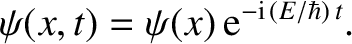
they are usually written
The probability of finding the particle between
. For this reason,
they are usually written
The probability of finding the particle between  and
and  at time
  is
is
 |
(4.70) |
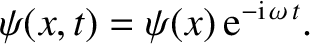
 is called a stationary
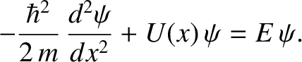
wavefunction. Substituting (4.69) into Schrödinger's equation, (4.22), we
obtain the following differential equation for ;
This equation is called the time-independent Schrödinger equation.
is called a stationary
wavefunction. Substituting (4.69) into Schrödinger's equation, (4.22), we
obtain the following differential equation for ;
This equation is called the time-independent Schrödinger equation.