General Interaction Between Macrosystems

Consider two systems, $A$ and $A'$ , that can interact by exchanging heat energy and doing work on one another. Let the system $A$ have energy $E$ , and adjustable external parameters $x_1, \cdots, x_n$ . Likewise, let the system $A'$ have energy $E'$ , and adjustable external parameters $x_1',\cdots, x_n'$ . The combined system $A^{(0)} = A + A'$ is assumed to be isolated. It follows from the first law of thermodynamics that

$$E+E' = E^{ (0)} = {\rm constant}.$$ (5.42)

Thus, the energy $E'$ of system $A'$ is determined once the energy $E$ of system $A$ is given, and vice versa. In fact, $E'$ could be regarded as a function of $E$ . Furthermore, if the two systems can interact mechanically then, in general, the parameters $x'$ are some function of the parameters $x$ . As a simple example, if the two systems are separated by a movable partition, in an enclosure of fixed volume $V^{ (0)}$ , then

$$V + V' = V^{ (0)} = {\rm constant},$$ (5.43)

where $V$ and $V'$ are the volumes of systems $A$ and $A'$ , respectively.

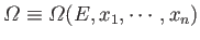
The total number of microstates accessible to $A^{(0)}$ is clearly a function of $E$ , and the parameters $x_\alpha$ (where $\alpha$ runs from 1 to $n$ ), so ${\mit\Omega}^{ (0)}\equiv {\mit\Omega}^{ (0)}(E, x_1, \cdots, x_n)$ . We have already demonstrated (in Section 5.2) that ${\mit\Omega}^{ (0)}$ exhibits a very pronounced maximum at one particular value of the energy, $E= \tilde{E}$ , when $E$ is varied but the external parameters are held constant. This behavior comes about because of the very strong,

$${\mit\Omega} \propto E^{ f},$$ (5.44)

increase in the number of accessible microstates of $A$ (or $A'$ ) with energy. However, according to Section 3.8, the number of accessible microstates exhibits a similar strong increase with the volume, which is a typical external parameter, so that

$${\mit\Omega} \propto V^{ f}.$$ (5.45)

It follows that the variation of ${\mit\Omega}^{ (0)}$ with a typical parameter, $x_\alpha$ , when all the other parameters and the energy are held constant, also exhibits a very sharp maximum at some particular value, $x_\alpha=\tilde{x}_\alpha$ . The equilibrium situation corresponds to the configuration of maximum probability, in which virtually all systems $A^{(0)}$ in the ensemble have values of $E$ and $x_\alpha$ very close to $\tilde{E}$ and $\tilde{x}_\alpha$ , respectively. The mean values of these quantities are thus given by $\overline{E}=\tilde{E}$ and $\bar{x}_\alpha= \tilde{x}_\alpha$ .

Consider a quasi-static process in which the system $A$ is brought from an equilibrium state described by $\overline{E}$ and $\bar{x}_\alpha$ to an infinitesimally different equilibrium state described by $\overline{E}+d\overline{E}$ and $\bar{x}_\alpha + d\bar{x}_\alpha$ . Let us calculate the resultant change in the number of microstates accessible to $A$ . Because ${\mit\Omega}\equiv {\mit\Omega}(E, x_1,\cdots, x_n)$ , the change in $\ln{\mit\Omega}$ follows from standard mathematics:

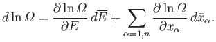$$d \ln {\mit\Omega} = \frac{\partial \ln {\mit\Omega}}{\partial E}... ...alpha=1,n}\frac{\partial \ln {\mit\Omega}}{\partial x_\alpha} d\bar{x}_\alpha.$$ (5.46)

However, we have previously demonstrated that

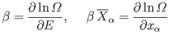$$\beta = \frac{\partial \ln {\mit\Omega}}{\partial E},    \beta \overline{X}_\alpha =\frac{\partial\ln {\mit\Omega}}{\partial x_\alpha}$$ (5.47)

[in Equations (5.30) and (5.41), respectively], so Equation (5.46) can be written

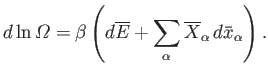$$d\ln{\mit\Omega} = \beta\left(d\overline{E} + \sum_\alpha \overline{X}_\alpha d\bar{x}_\alpha \right).$$ (5.48)

Note that the temperature parameter, $\beta$ , and the mean conjugate forces, $\overline{X}_\alpha$ , are only well defined for equilibrium states. This is why we are only considering quasi-static changes in which the two systems are always arbitrarily close to equilibrium.

Let us rewrite Equation (5.48) in terms of the thermodynamic temperature, $T$ , using the relation $\beta\equiv 1/k T$ . We obtain

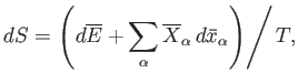$$d S = \left.\left(d\overline{E} +\sum_\alpha \overline{X}_\alpha d\bar{x}_\alpha\right)\right/T,$$ (5.49)

where

$$S = k\ln{\mit\Omega}.$$ (5.50)

Equation (5.49) is a differential relation that enables us to calculate the quantity $S$ as a function of the mean energy, $\overline{E}$ , and the mean external parameters, $\bar{x}_\alpha$ , assuming that we can calculate the temperature, $T$ , and mean conjugate forces, $\overline{X}_\alpha$ , for each equilibrium state. The function $S(\overline{E}, \bar{x}_\alpha)$ is termed the entropy of system $A$ . The word entropy is derived from the Greek entrope, which means ``a turning towards" or "tendency." The reason for this etymology will become apparent presently. It can be seen from Equation (5.50) that the entropy is merely a parameterization of the number of accessible microstates. Hence, according to statistical mechanics, $S(\overline{E}, \bar{x}_\alpha)$ is essentially a measure of the relative probability of a state characterized by values of the mean energy and mean external parameters $\overline{E}$ and $\bar{x}_\alpha$ , respectively.

According to Equation (4.16), the net amount of work performed during a quasi-static change is given by

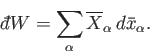$${\mathchar'26\mkern-11mud}W = \sum_\alpha \overline{X}_\alpha d\bar{x}_\alpha.$$ (5.51)

It follows from Equation (5.49) that

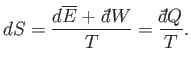$$d S = \frac{d\overline{E} + {\mathchar'26\mkern-11mud}W}{T} =\frac{ {\mathchar'26\mkern-11mud}Q}{T}.$$ (5.52)

Thus, the thermodynamic temperature, $T$ , is the integrating factor for the first law of thermodynamics,

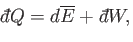$${\mathchar'26\mkern-11mud}Q = d\overline{E} + {\mathchar'26\mkern-11mud}W,$$ (5.53)

which converts the inexact differential ${\mathchar'26\mkern-11mud}Q$ into the exact differential $dS$ . (See Section 4.5.) It follows that the entropy difference between any two macrostates $i$ and $f$ can be written

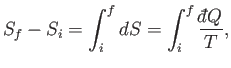$$S_f - S_i = \int_i^f dS = \int_i^f \frac{{\mathchar'26\mkern-11mud}Q}{T},$$ (5.54)

where the integral is evaluated for any process through which the system is brought quasi-statically via a sequence of near-equilibrium configurations from its initial to its final macrostate. The process has to be quasi-static because the temperature, $T$ , which appears in the integrand, is only well defined for an equilibrium state. Because the left-hand side of the previous equation only depends on the initial and final states, it follows that the integral on the right-hand side is independent of the particular sequence of quasi-static changes used to get from $i$ to $f$ . Thus, $\int_i^f {\mathchar'26\mkern-11mud}Q/T$ is independent of the process (provided that it is quasi-static).

All of the concepts that we have encountered up to now in this course, such as temperature, heat, energy, volume, pressure, et cetera, have been fairly familiar to us from other branches of physics. However, entropy, which turns out to be of crucial importance in thermodynamics, is something quite new. Let us consider the following questions. What does the entropy of a thermodynamic system actually signify? What use is the concept of entropy?