


Next: Properties of Entropy
Up: Statistical Thermodynamics
Previous: General Interaction Between Macrosystems
Entropy
Consider an isolated system whose energy is known to lie in a narrow range.
Let
 be the number of accessible microstates. According to the principle
of equal a priori probabilities, the system is equally likely
to be found in any one of these states when it is in
thermal equilibrium. The accessible states are just that set
of microstates that are consistent with the macroscopic constraints imposed on the
system. These constraints can usually be quantified by specifying the values
of some parameters,
be the number of accessible microstates. According to the principle
of equal a priori probabilities, the system is equally likely
to be found in any one of these states when it is in
thermal equilibrium. The accessible states are just that set
of microstates that are consistent with the macroscopic constraints imposed on the
system. These constraints can usually be quantified by specifying the values
of some parameters,
 , that characterize the
macrostate. Note that these parameters are not necessarily external in nature. For example,
we could specify
either the volume (an external parameter) or the mean pressure
(the mean force conjugate to the volume).
The number of accessible states is clearly a function of the chosen
parameters, so we can write
, that characterize the
macrostate. Note that these parameters are not necessarily external in nature. For example,
we could specify
either the volume (an external parameter) or the mean pressure
(the mean force conjugate to the volume).
The number of accessible states is clearly a function of the chosen
parameters, so we can write
 for the number of
microstates consistent with a macrostate in which the general parameter
for the number of
microstates consistent with a macrostate in which the general parameter
 lies in the range
to
lies in the range
to
 .
.
Suppose that we start from a system in thermal equilibrium.
According to statistical mechanics, each of the
 ,
say, accessible states are equally likely. Let us now remove, or relax, some of the
constraints imposed on the system. Clearly, all of the microstates formally
accessible to the system are still accessible, but many additional states will,
in general, become accessible. Thus, removing or relaxing constraints can only have
the effect of increasing, or possibly leaving unchanged, the number of
microstates accessible to the system. If the final number of accessible states
is
,
say, accessible states are equally likely. Let us now remove, or relax, some of the
constraints imposed on the system. Clearly, all of the microstates formally
accessible to the system are still accessible, but many additional states will,
in general, become accessible. Thus, removing or relaxing constraints can only have
the effect of increasing, or possibly leaving unchanged, the number of
microstates accessible to the system. If the final number of accessible states
is
 then we can write
 |
(5.55) |
Immediately after the constraints are relaxed, the systems in the ensemble
are
not in any of the microstates from which they were previously excluded. So, the
systems only occupy a fraction
 |
(5.56) |
of the
states now accessible to them. This is clearly not a equilibrium
situation. Indeed, if
 then the configuration
in which the systems
are only distributed over the original
states is an extremely unlikely
one.
In fact, its probability of occurrence is given by Equation (5.56). According to the
then the configuration
in which the systems
are only distributed over the original
states is an extremely unlikely
one.
In fact, its probability of occurrence is given by Equation (5.56). According to the
 -theorem (see Section 3.4), the ensemble will evolve in time until a more probable
final state is reached in
which the systems are evenly distributed over the
available states.
-theorem (see Section 3.4), the ensemble will evolve in time until a more probable
final state is reached in
which the systems are evenly distributed over the
available states.
As a simple example, consider a system
consisting of a box divided into two regions of equal volume. Suppose that,
initially, one region is filled with gas, and the other is empty. The constraint
imposed on the system is, thus, that the coordinates of all of the gas molecules must
lie within the filled region. In other words, the volume accessible to the
system is  , where
  is half the volume of the box. The constraints
imposed on the system can be relaxed by removing the partition, and allowing gas to
flow into both regions. The volume accessible to the gas is now
is half the volume of the box. The constraints
imposed on the system can be relaxed by removing the partition, and allowing gas to
flow into both regions. The volume accessible to the gas is now
 .
Immediately after the partition is removed, the system is
in an extremely improbable state.
We know, from Section 3.8, that, at constant energy, the variation of the number
of accessible states of an ideal gas with the volume is
.
Immediately after the partition is removed, the system is
in an extremely improbable state.
We know, from Section 3.8, that, at constant energy, the variation of the number
of accessible states of an ideal gas with the volume is
 |
(5.57) |
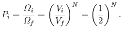
where  is the number of particles. Thus, the probability of observing the state
immediately after the partition is removed in an ensemble of equilibrium
systems with
volume
is the number of particles. Thus, the probability of observing the state
immediately after the partition is removed in an ensemble of equilibrium
systems with
volume  is
is
 |
(5.58) |
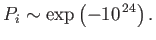
If the box contains of order 1 mole of molecules then
 , and this
probability is fantastically small:
, and this
probability is fantastically small:
 |
(5.59) |
Clearly, the system will evolve towards a more probable state.
This discussion can also be phrased in terms of
the parameters,
, of the system.
Suppose that a constraint is removed.
For instance, one of the parameters,  , say, which originally had the value
 , is now allowed to vary. According to statistical mechanics, all states
accessible to the system are equally likely. So, the probability
, is now allowed to vary. According to statistical mechanics, all states
accessible to the system are equally likely. So, the probability  of finding the
system in equilibrium with the parameter
in the range
to
of finding the
system in equilibrium with the parameter
in the range
to
 is proportional
to the number of microstates in this interval: that is,
is proportional
to the number of microstates in this interval: that is,
 |
(5.60) |
Usually,
 has a very pronounced maximum at some particular
value
has a very pronounced maximum at some particular
value  .
(See Section 5.2.) This means that
practically all systems in the final equilibrium ensemble
have values of
close to
. Thus, if
.
(See Section 5.2.) This means that
practically all systems in the final equilibrium ensemble
have values of
close to
. Thus, if
 ,
initially,
then the parameter
will change until it attains a final
value close to
,
where
is maximum. This discussion can be summed up in a single
phrase:
,
initially,
then the parameter
will change until it attains a final
value close to
,
where
is maximum. This discussion can be summed up in a single
phrase:
If some of the constraints of an isolated system are removed then the parameters
of the system tend to readjust themselves in such a way that
Suppose that the final equilibrium state has been reached, so that the systems in the
ensemble are uniformly distributed over the
accessible final states.
If the original constraints are reimposed then the systems
in the ensemble still
occupy these
states with equal probability. Thus, if
 then simply restoring the constraints does not restore the initial situation.
Once the systems are randomly distributed over the
states, they cannot
be expected to spontaneously move out of some of these states, and occupy a
more restricted class of states, merely in
response to the reimposition of a constraint.
The initial condition can also not be restored by removing further constraints. This
could only lead to even more states becoming accessible to the system.
then simply restoring the constraints does not restore the initial situation.
Once the systems are randomly distributed over the
states, they cannot
be expected to spontaneously move out of some of these states, and occupy a
more restricted class of states, merely in
response to the reimposition of a constraint.
The initial condition can also not be restored by removing further constraints. This
could only lead to even more states becoming accessible to the system.
Suppose that a process occurs in which an isolated system
goes from some initial configuration to some final configuration. If the
final configuration is such that the imposition or removal of constraints
cannot by itself restore the initial condition then
the process is deemed irreversible. On the other hand, if it is such that the
imposition or removal of constraints can restore the initial condition
then the
process is deemed reversible. From what we have already said, an irreversible
process is clearly one in which the removal of constraints leads to a situation
where
. A reversible process corresponds to the special
case where the removal of constraints does not change the number of accessible
states, so that
 . In this situation, the systems
remain
distributed with equal probability over these states irrespective of whether the
constraints are imposed or not.
. In this situation, the systems
remain
distributed with equal probability over these states irrespective of whether the
constraints are imposed or not.
Our microscopic definition of irreversibility is in accordance with the
macroscopic definition discussed in Section 3.6. Recall that, on a
macroscopic level, an irreversible process is one that ``looks unphysical''
when viewed in reverse. On a microscopic level, it is clearly plausible that a
system should spontaneously evolve from an improbable to a probable configuration
in response to the relaxation of some constraint. However, it is quite manifestly
implausible that a system should ever spontaneously evolve from a probable
to an improbable configuration. Let us consider our example again.
If a gas is initially
restricted to one half of a box, via a partition, then the flow of gas
from one side of the box to the other when the partition is removed is an
irreversible process. This process is irreversible on a microscopic level because the
initial configuration cannot be recovered by simply replacing the partition.
It is irreversible on a macroscopic level because it is obviously
unphysical for the molecules of a gas to spontaneously distribute themselves
in such a manner that
they only occupy half of the available volume.
It is actually possible to quantify irreversibility.
In other words, in addition to
stating that
a given process is irreversible, we can also give some indication
of how irreversible it is. The parameter that measures irreversibility is
the number of accessible states,
.
Thus, if
for an isolated
system spontaneously
increases then the process is irreversible, the degree of irreversibility
being proportional to the amount of
the increase. If
stays the same then the process
is reversible. Of course, it is unphysical for
to ever spontaneously
decrease. In symbols, we can write
 |
(5.61) |
for any physical process operating on an isolated system.
In practice,
itself is a rather unwieldy parameter
with which to measure
irreversibility. For instance, in the previous
example, where an ideal gas doubles in
volume (at constant energy)
due to the removal of a partition, the fractional increase in
is
 |
(5.62) |
where  is the number of moles. This is an extremely large number.
It is far more convenient to measure irreversibility in terms of
is the number of moles. This is an extremely large number.
It is far more convenient to measure irreversibility in terms of
 .
If Equation (5.61) is true then it is certainly also true that
.
If Equation (5.61) is true then it is certainly also true that
 |
(5.63) |
for any physical process operating on an isolated system.
The increase in
when an ideal gas doubles
in volume (at constant energy) is
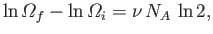 |
(5.64) |
where
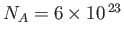 . This is a far more manageable
number. Because we usually deal with particles by the mole in laboratory
physics, it makes sense to pre-multiply our measure of irreversibility by a
number of order
. This is a far more manageable
number. Because we usually deal with particles by the mole in laboratory
physics, it makes sense to pre-multiply our measure of irreversibility by a
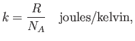
number of order  . For historical reasons, the number that is
generally used for this purpose is the Boltzmann constant,
. For historical reasons, the number that is
generally used for this purpose is the Boltzmann constant,  , which can be written
 |
(5.65) |
where
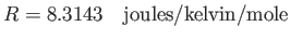 |
(5.66) |
is the ideal gas constant that appears in the well-known equation of state for
an ideal gas,
 . Thus, the final form for our measure of irreversibility
is
. Thus, the final form for our measure of irreversibility
is
 |
(5.67) |
This quantity is termed ``entropy'', and is measured in joules per degree kelvin.
The increase in entropy when an ideal gas doubles in volume (at constant
energy) is
 |
(5.68) |
which is order unity for laboratory-scale systems (i.e., those containing about
one mole of particles). The essential irreversibility of macroscopic phenomena
can be summed up as follows:
 |
(5.69) |
for a process acting on an isolated system. [This formula is equivalent to
Equations (5.61) and (5.63).] Thus:
The entropy of an isolated
system tends to increase with time, and can never decrease.
This
proposition is known
as the second law of thermodynamics.
One way of thinking of the number of accessible states,
,
is that it is a measure
of the disorder associated with a macrostate. For a system exhibiting
a high degree of order, we would expect a strong correlation between the motions
of the individual particles. For instance, in a fluid there might be a strong tendency
for the particles to move in one particular direction, giving rise to
an ordered flow of the
system in that direction.
On the other hand, for a system exhibiting a low degree of order, we expect
far less correlation between the motions of individual particles. It follows that,
all other things being equal, an ordered system is more constrained than a disordered
system, because the former is excluded from microstates in which there is not
a strong correlation between individual particle motions, whereas the latter is not.
Another way of saying this is that an ordered system has less accessible microstates
than a corresponding disordered system. Thus, entropy is
effectively a measure of the disorder
in a system (the disorder increases with increasing  ).
With this interpretation, the second law of thermodynamics reduces to the statement
that isolated systems tend to become more disordered with time, and can never
become more ordered.
).
With this interpretation, the second law of thermodynamics reduces to the statement
that isolated systems tend to become more disordered with time, and can never
become more ordered.
Note that the second law of thermodynamics only applies to isolated
systems. The
entropy of a non-isolated system can decrease. For instance, if a gas expands
(at constant energy) to twice its initial volume
after the removal of a partition, we can subsequently recompress
the gas to its original volume. The energy of the gas will increase because of the
work done on it during compression, but if we absorb some heat from the gas then we
can restore it to its initial state. Clearly, in restoring the gas to its original
state, we have restored its original entropy.
This appears to violate the second law of thermodynamics, because the entropy
should have increased in what is obviously an irreversible process. However,
if we consider a new system consisting
of the gas plus the compression and heat absorption machinery then it is still
true that the entropy of this system (which is assumed to be isolated)
must increase in time. Thus, the entropy of the gas is only kept the same at the
expense of increasing the entropy of the rest of the system, and the total
entropy is increased. If we consider the system of everything in the universe, which
is certainly an isolated system because there is nothing outside it with which it could
interact, then the second law of thermodynamics becomes:
The disorder of the universe tends to increase with time, and can never decrease.
Next: Properties of Entropy
Up: Statistical Thermodynamics
Previous: General Interaction Between Macrosystems
Richard Fitzpatrick
2016-01-25