| (3.4) |
| (3.5) |
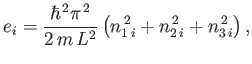
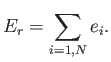
For example, consider ![]() non-interacting spinless particles
of mass
non-interacting spinless particles
of mass ![]() confined in a cubic box of dimension
confined in a cubic box of dimension ![]() . According to standard
wave-mechanics, the
energy levels of the
. According to standard
wave-mechanics, the
energy levels of the ![]() th particle are given by
th particle are given by
 |
(3.6) |
 |
(3.7) |
Consider, now, a statistical ensemble of systems made up of weakly-interacting particles. Suppose that this ensemble is initially very far from equilibrium. For instance, the systems in the ensemble might only be distributed over a very small subset of their accessible states. If each system starts off in a particular stationary state (i.e., with a particular set of quantum numbers) then, in the absence of particle interactions, it will remain in that state for ever. Hence, the ensemble will always stay far from equilibrium, and the principle of equal a priori probabilities will never be applicable. In reality, particle interactions cause each system in the ensemble to make transitions between its accessible ``stationary'' states. This allows the overall state of the ensemble to change in time.
Let us label the accessible states of our system by the index ![]() . We can
ascribe a time-dependent probability,
. We can
ascribe a time-dependent probability, ![]() , of finding the system
in a particular approximate stationary
state
, of finding the system
in a particular approximate stationary
state ![]() at time
at time ![]() . Of course,
. Of course, ![]() is proportional
to the number of systems in the ensemble in state
is proportional
to the number of systems in the ensemble in state ![]() at time
at time ![]() . In general,
. In general,
![]() is time-dependent because the ensemble is evolving towards an
equilibrium state. Let us assume that the probabilities are properly
normalized, so that the sum over all accessible states always yields unity: that is,
is time-dependent because the ensemble is evolving towards an
equilibrium state. Let us assume that the probabilities are properly
normalized, so that the sum over all accessible states always yields unity: that is,
 |
(3.8) |
Small interactions between particles cause transitions between the approximate
stationary states of the system. Thus, there exists some transition probability
per unit time, ![]() , that a system originally in state
, that a system originally in state ![]() ends up in state
ends up in state
![]() as a result of these interactions. Likewise, there exists a probability
per unit time
as a result of these interactions. Likewise, there exists a probability
per unit time ![]() that a system in state
that a system in state ![]() makes a transition to
state
makes a transition to
state ![]() . These transition probabilities are meaningful in quantum mechanics
provided that the particle interaction strength is sufficiently small, there is
a nearly continuous distribution of accessible energy levels, and we consider time
intervals that are not too small. These conditions are easily satisfied for
the types of systems usually analyzed via statistical mechanics (e.g.,
nearly-ideal gases). One important conclusion of quantum
mechanics is that the forward and backward transition probabilities between two
states are the same, so that
. These transition probabilities are meaningful in quantum mechanics
provided that the particle interaction strength is sufficiently small, there is
a nearly continuous distribution of accessible energy levels, and we consider time
intervals that are not too small. These conditions are easily satisfied for
the types of systems usually analyzed via statistical mechanics (e.g.,
nearly-ideal gases). One important conclusion of quantum
mechanics is that the forward and backward transition probabilities between two
states are the same, so that
Suppose that we were to ``film'' a microscopic process, such as two classical particles approaching one another, colliding, and moving apart. We could then gather an audience together and show them the film. To make things slightly more interesting we could play it either forwards or backwards. Because of the time-reversal symmetry of classical mechanics, the audience would not be able to tell which way the film was running. In both cases, the film would show completely plausible physical events.
We can play the same game for a quantum process. For instance, we could ``film'' a group of photons impinging on some atoms. Occasionally, one of the atoms will absorb a photon and make a transition to an excited state (i.e., a state with higher than normal energy). We could easily estimate the rate constant for this process by watching the film carefully. If we play the film backwards then it will appear to show excited atoms occasionally emitting a photon, and then decaying back to their unexcited state. If quantum mechanics possesses time-reversal symmetry (which it certainly does) then both films should appear equally plausible. This means that the rate constant for the absorption of a photon to produce an excited state must be the same as the rate constant for the excited state to decay by the emission of a photon. Otherwise, in the backwards film, the excited atoms would appear to emit photons at the wrong rate, and we could then tell that the film was being played backwards. It follows, therefore, that, as a consequence of time-reversal symmetry, the rate constant for any process in quantum mechanics must equal the rate constant for the inverse process.
The probability, ![]() , of finding the systems in the ensemble
in a particular state
, of finding the systems in the ensemble
in a particular state ![]() changes
with time for two reasons. Firstly, systems in another state
changes
with time for two reasons. Firstly, systems in another state ![]() can make transitions
to the state
can make transitions
to the state ![]() . The rate at which this occurs is
. The rate at which this occurs is ![]() , the probability
that the systems are in the state
, the probability
that the systems are in the state ![]() to begin with, multiplied by the rate constant
of the transition
to begin with, multiplied by the rate constant
of the transition ![]() . Secondly, systems in the state
. Secondly, systems in the state ![]() can make
transitions to other states such as
can make
transitions to other states such as ![]() . The rate at which this occurs
is clearly
. The rate at which this occurs
is clearly ![]() times
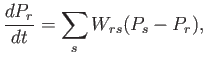
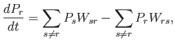
times ![]() . We can, thus, write a simple differential equation
for the time evolution of
. We can, thus, write a simple differential equation
for the time evolution of ![]() :
:
 |
(3.10) |
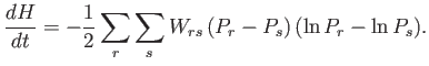
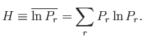
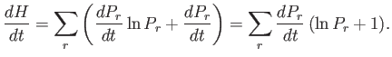
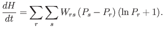
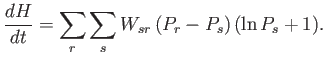
Consider now the quantity ![]() (from which the
(from which the ![]() -theorem derives its name),
which is defined as the average value of
-theorem derives its name),
which is defined as the average value of ![]() taken over all accessible states:
taken over all accessible states:
 |
(3.12) |
 |
(3.13) |
 |
(3.14) |
 |
(3.15) |
 |
(3.17) |
The ![]() -theorem tells us that if an isolated system is initially not in
equilibrium then it will evolve in time, under the influence of particle interactions, in
such a manner that the quantity
-theorem tells us that if an isolated system is initially not in
equilibrium then it will evolve in time, under the influence of particle interactions, in
such a manner that the quantity ![]() always decreases. This process will
continue until
always decreases. This process will
continue until ![]() reaches its minimum possible value, at which point
reaches its minimum possible value, at which point
![]() , and there is no further evolution of the
system. According to Equation (3.16), in this final equilibrium state,
the system is equally likely to be found in any one of its accessible
states. This is, of course, the situation predicted by the principle
of equal a priori probabilities.
, and there is no further evolution of the
system. According to Equation (3.16), in this final equilibrium state,
the system is equally likely to be found in any one of its accessible
states. This is, of course, the situation predicted by the principle
of equal a priori probabilities.
The previous argument does not constitute a mathematically
rigorous proof that the principle of equal a priori probabilities
applies to many-particle systems, because we
tacitly made an unwarranted
assumption. That is, we assumed
that the probability of the system making a transition
from some state ![]() to another state
to another state ![]() is independent of the past history
of the system. In general, this is not the case in physical
systems, although there are many
situations in which it is a fairly good approximation. Thus, the
epistemological status of the principle of equal a priori probabilities is that it
is plausible, but remains unproven. As we have already mentioned,
the ultimate justification for this principle is empirical--it leads to theoretical predictions that are in accordance with
experimental observations.
is independent of the past history
of the system. In general, this is not the case in physical
systems, although there are many
situations in which it is a fairly good approximation. Thus, the
epistemological status of the principle of equal a priori probabilities is that it
is plausible, but remains unproven. As we have already mentioned,
the ultimate justification for this principle is empirical--it leads to theoretical predictions that are in accordance with
experimental observations.