Pauli Two-Component Formalism

We have seen, in Section 4.4, that the eigenstates of orbital angular momentum can be conveniently represented as spherical harmonics. In this representation, the orbital angular momentum operators take the form of differential operators involving only angular coordinates. On the other hand, it is conventional to represent the eigenstates of spin angular momentum as column (or row) matrices. In this representation, the spin angular momentum operators take the form of matrices.

The matrix representation of a spin one-half system was introduced by Pauli in 1927 [80]. Recall, from Section 5.4, that a general spin ket can be expressed as a linear combination of the two eigenkets of $S_z$ belonging to the eigenvalues $\pm \hbar/2$ . These are denoted $\vert\pm \rangle$ . Let us represent these basis eigenkets as column vectors:

$$\vert+\rangle \rightarrow \left(\!\begin{array}{c}1\\ 0\end{array}\!\right) \equiv \chi_+,$$ (5.57)

$$\vert-\rangle \rightarrow \left(\!\begin{array}{c}0\\ 1\end{array}\!\right) \equiv \chi_-.$$ (5.58)

The corresponding eigenbras are represented as row vectors:

$$\langle +\vert \rightarrow (1, 0) \equiv \chi_+^{\dag },$$ (5.59)

$$\langle - \vert \rightarrow (0, 1) \equiv \chi_-^{\dag }.$$ (5.60)

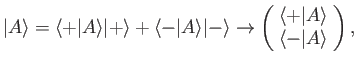
In this scheme, a general ket takes the form

$$\vert A\rangle = \langle +\vert A\rangle \vert+\rangle + \langle ... ...array}{c}\langle +\vert A\rangle\\ \langle -\vert A\rangle\end{array}\!\right),$$ (5.61)

and a general bra becomes

$$\langle A\vert =\langle A\vert+\rangle \langle +\vert + \langle A... ...le \langle -\vert \rightarrow (\langle A\vert+\rangle, \langle A\vert-\rangle).$$ (5.62)

The column vector (5.61) is called a two-component spinor, and can be written

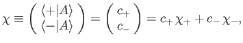$$\chi \equiv \left(\!\begin{array}{c}\langle +\vert A\rangle\\ \la... ...!\begin{array}{c} c_+\\ c_- \end{array}\!\right) = c_+\, \chi_+ + c_- \,\chi_-,$$ (5.63)

where the $c_\pm$ are complex numbers. The row vector (5.62) becomes

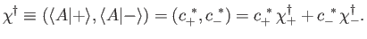$$\chi^{\dag } \equiv (\langle A\vert+\rangle, \langle A\vert-\rang... ...ast}, c_-^{~\ast}) =c_+^{~\ast}\, \chi_+^{\dag } + c_-^{~\ast}\,\chi_-^{\dag }.$$ (5.64)

Consider the ket obtained by the action of a spin operator on ket $A$ :

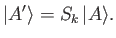$$\vert A'\rangle = S_k \,\vert A\rangle.$$ (5.65)

This ket is represented as

$$\vert A'\rangle \rightarrow \left(\!\begin{array}{c}\langle +\vert A'\rangle\\ \langle -\vert A'\rangle\end{array}\!\right)\equiv \chi'.$$ (5.66)

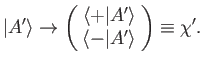
However,

$$\langle + \vert A'\rangle = \langle + \vert\,S_k\,\vert +\rangle \langle +\vert A\rangle + \langle +\vert\,S_k\, \vert-\rangle \langle -\vert A\rangle,$$ (5.67)

$$\langle - \vert A'\rangle = \langle - \vert\,S_k\,\vert +\rangle \langle +\vert A\rangle + \langle -\vert\,S_k\, \vert-\rangle \langle -\vert A\rangle,$$ (5.68)

or

$$\left(\!\begin{array}{c}\langle +\vert A'\rangle\\ [0.5ex] \langl... ...}\langle +\vert A\rangle\\ [0.5ex] \langle -\vert A\rangle\end{array}\!\right).$$ (5.69)

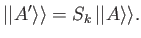
It follows that we can represent the operator/ket relation (5.65) as the matrix relation

$$\chi' =\left( \frac{\hbar}{2}\right)\sigma_k \,\chi,$$ (5.70)

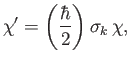
where the $\sigma_k$ are the matrices of the $\langle \pm \vert\,S_k\,\vert\pm \rangle$ values divided by $\hbar/2$ . These matrices, which are called the Pauli matrices, can easily be evaluated using the explicit forms for the spin operators given in Equations (5.11)-(5.13). We find that

$$\sigma_1 = \left(\!\begin{array}{rr} 0, &1\\ 1,&0\end{array}\!\right),$$ (5.71)

$$\sigma_2 = \left(\!\begin{array}{rr} 0, &-{\rm i}\\ {\rm i},&0\end{array}\!\right),$$ (5.72)

$$\sigma_3 = \left(\!\begin{array}{rr} 1, &0\\ 0,&-1\end{array}\!\right).$$ (5.73)

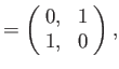
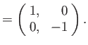
Here, 1, 2, and 3 refer to $x$ , $y$ , and $z$ , respectively. Note that, in this scheme, we are effectively representing the spin operators in terms of the Pauli matrices:

$$S_k \rightarrow \left(\frac{\hbar}{2} \right)\sigma_k.$$ (5.74)

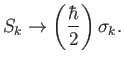
The expectation value of $S_k$ can be written in terms of spinors and the Pauli matrices:

$$\langle S_k \rangle = \langle A\vert\,S_k \,\vert A\rangle = \sum... ...\vert A\rangle = \left(\frac{\hbar}{2}\right) \,\chi^{\dag }\, \sigma_k\, \chi.$$ (5.75)

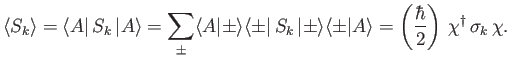
The fundamental commutation relation for angular momentum, Equation (5.1), can be combined with Equation (5.74) to give the following commutation relation for the Pauli matrices:

$$\mbox{\boldmath$\sigma$} \times \mbox{\boldmath$\sigma$} = 2\,{\rm i}\, \mbox{\boldmath$\sigma$} .$$ (5.76)

It is easily seen that the matrices (5.71)-(5.73) actually satisfy these relations (i.e., $\sigma_1\, \sigma_2 - \sigma_2\,\sigma_1 = 2\,{\rm i} \,\sigma_3$ , plus all cyclic permutations). (See Exercise 3.) It is also easily seen that the Pauli matrices satisfy the anti-commutation relations

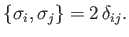$$\{ \sigma_i, \sigma_j \} = 2 \,\delta_{ij}.$$ (5.77)

(See Exercise 3.) Here, $\{a,b\}\equiv a\,b+b\,a$ .

Let us examine how the Pauli scheme can be extended to take into account the position of a spin one-half particle. Recall, from Section 5.3, that we can represent a general basis ket as the product of basis kets in position space and spin space:

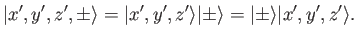$$\vert x', y', z', \pm\rangle = \vert x', y', z'\rangle\vert \pm\rangle = \vert \pm\rangle \vert x', y', z'\rangle.$$ (5.78)

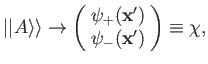
The ket corresponding to state $A$ is denoted $\vert\vert A\rangle\rangle$ , and resides in the product space of the position and spin ket spaces. State $A$ is completely specified by the two wavefunctions

$$\psi_+(x', y', z') = \langle x', y', z' \vert\langle +\vert\vert A\rangle\rangle,$$ (5.79)

$$\psi_-(x', y', z') = \langle x', y', z' \vert\langle -\vert\vert A\rangle\rangle.$$ (5.80)

Consider the operator relation

$$\vert\vert A'\rangle\rangle = S_k\, \vert\vert A\rangle\rangle.$$ (5.81)

It is easily seen that

$$\langle x', y', z'\vert \langle +\vert A'\rangle\rangle = \langle + \vert\,S_k\, \vert+\rangle \langle x',y',z'\vert\lang... ...\,S_k \,\vert-\rangle \langle x',y',z'\vert\langle -\vert\vert A\rangle\rangle,$$ (5.82)

$$\langle x', y', z'\vert \langle -\vert A'\rangle\rangle = \langle - \vert\,S_k \,\vert+\rangle \langle x',y',z'\vert\lang... ...\,S_k\, \vert-\rangle \langle x',y',z'\vert\langle -\vert\vert A\rangle\rangle,$$ (5.83)

where use has been made of the fact that the spin operator $S_k$ commutes with the eigenbras $\langle x', y', z'\vert$ . It is fairly obvious that we can represent the operator relation (5.81) as a matrix relation if we generalize our definition of a spinor by writing

$$\vert\vert A\rangle\rangle \rightarrow \left(\! \begin{array}{c}\psi_+({\bf x}') \\ \psi_-({\bf x}')\end{array}\!\right)\equiv \chi,$$ (5.84)

and so on. The components of the spinor are now wavefunctions, instead of complex numbers. We shall refer to such a construct as a spinor-wavefunction. In this scheme, the operator equation (5.81) becomes simply

$$\chi' = \left(\frac{\hbar}{2}\right) \sigma_k \,\chi.$$ (5.85)

Consider the operator relation

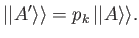$$\vert\vert A'\rangle\rangle = p_k\, \vert\vert A\rangle\rangle.$$ (5.86)

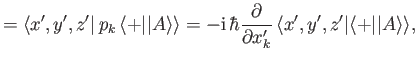
In the Schrödinger representation, we have

$$\langle x', y', z'\vert \langle +\vert A'\rangle\rangle = \langle x', y', z'\vert\,p_k\, \langle +\vert\vert A\rangle\ran... ... {\partial x_k'}\, \langle x', y', z'\vert \langle +\vert\vert A\rangle\rangle,$$ (5.87)

$$\langle x', y', z'\vert \langle -\vert A'\rangle\rangle = \langle x', y', z'\vert\,p_k\, \langle -\vert\vert A\rangle\ran... ... {\partial x_k'}\, \langle x', y', z'\vert \langle -\vert\vert A\rangle\rangle,$$ (5.88)

where use has been made of Equation (2.78). The previous equation reduces to

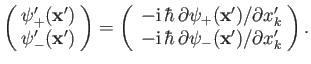$$\left(\! \begin{array}{c} \psi_+'({\bf x}')\\ \psi_-' ({\bf x}') ... ... -{\rm i}\,\hbar \,\partial \psi_-({\bf x}')/\partial x_k'\end{array}\!\right).$$ (5.89)

Thus, the operator equation (5.86) can be written

$$\chi' = p_k\, \chi,$$ (5.90)

where

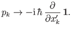$$p_k \rightarrow -{\rm i}\,\hbar\,\frac{\partial}{\partial x_k'}\, {\bf 1}.$$ (5.91)

Here, ${\bf 1}$ is the $2\times 2$ unit matrix. In fact, any position operator (e.g., $p_k$ or $L_k$ ) is represented in the Pauli scheme as some differential operator of the position eigenvalues multiplied by the $2\times 2$ unit matrix.

What about combinations of position and spin operators? The most commonly occurring combination is a dot product: for instance, ${\bf S}\cdot {\bf L} = (\hbar/2)\,$$\sigma$ $\cdot {\bf L}$ . Consider the hybrid operator $\sigma$ $\cdot {\bf a}$ , where ${\bf a} \equiv (a_x, a_y, a_z)$ is some vector position operator. This quantity is represented as a $2\times 2$ matrix:

$$\mbox{\boldmath$\sigma$} \cdot {\bf a} \equiv \sum_k a_k \,\sigma_k = \left(\!\begin{array... ... & a_1 -{\rm i}\,a_2\\ [0.5ex] a_1 + {\rm i}\,a_2, & -a_3 \end{array}\!\right).$$ (5.92)

Because, in the Schrödinger representation, a general position operator takes the form of a differential operator in $x'$ , $y'$ , or $z'$ , it is clear that the previous quantity must be regarded as a matrix differential operator that acts on spinor-wavefunctions of the general form (5.84).

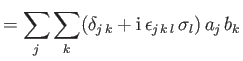
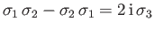
Finally, the important identity

$$( \mbox{\boldmath$\sigma$} \cdot {\bf a} ) \,( \mbox{\boldmath$\sigma$} \cdot {\bf b}) = {\bf a} \cdot {\bf b} +{\rm i}\, \mbox{\boldmath$\sigma$} \cdot ({\bf a} \times {\bf b} )$$ (5.93)

follows from the commutation and anti-commutation relations (5.76) and (5.77). In fact,

$$\sum_j \sigma_j \,a_j \sum_k \sigma_k \,b_k = \sum_j \sum_k \left(\frac{1}{2}\, \{\sigma_j, \sigma_k\} + \frac{1}{2} [\sigma_j, \sigma_k]\right) a_j \,b_k$$

$$= \sum_j \sum_k (\delta_{j\,k} + {\rm i}\,\epsilon_{j\,k\,l} \,\sigma_l)\,a_j \,b_k$$

$$= {\bf a} \cdot {\bf b} +{\rm i}\, \mbox{\boldmath$\sigma$} \cdot ({\bf a} \times {\bf b} ).$$ (5.94)