


Next: Magnetic Moments
Up: Spin Angular Momentum
Previous: Wavefunction of Spin One-Half
Rotation Operators in Spin Space
Let us, for the moment, forget about the spatial position of our spin one-half particle,
and concentrate on its spin state. A general
spin state  is represented by the ket
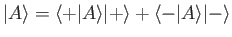 |
(5.23) |
in spin space.
In Section 4.3, we were able to construct an operator
 that
rotates the system through an angle
that
rotates the system through an angle
 about the
  -axis in position
space. Can we also construct an operator
-axis in position
space. Can we also construct an operator
 that rotates the
system through an angle
about the
-axis in spin space? By analogy
with Equation (4.62), we would expect such an operator to take the form
that rotates the
system through an angle
about the
-axis in spin space? By analogy
with Equation (4.62), we would expect such an operator to take the form
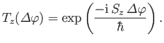 |
(5.24) |
Thus, after rotation, the ket  becomes
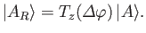 |
(5.25) |
To demonstrate that the operator (5.24) really does rotate the spin of the system,
let us consider its effect on
 . Under rotation, this
expectation value changes as follows:
. Under rotation, this
expectation value changes as follows:
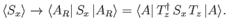 |
(5.26) |
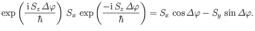
Thus, we need to compute
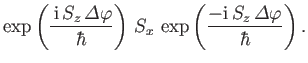 |
(5.27) |
This goal can be achieved in two different ways.
First, we can use the explicit formula for  given in Equation (5.11). We find
that expression (5.27) becomes
given in Equation (5.11). We find
that expression (5.27) becomes
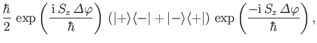 |
(5.28) |
or
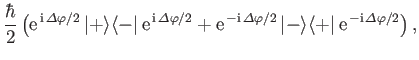 |
(5.29) |
which yields
 |
(5.30) |
where use has been made of Equations (5.11)-(5.13).
A second approach is to use the so-called Baker-Campbell-Hausdorff lemma [5,20,62]. This
takes the form
where  and
are operators, and
and
are operators, and  a real parameter. The proof
of this lemma is left as an exercise. (See Exercise 2.) Applying the Baker-Campbell-Hausdorff lemma
to expression (5.27), we obtain
a real parameter. The proof
of this lemma is left as an exercise. (See Exercise 2.) Applying the Baker-Campbell-Hausdorff lemma
to expression (5.27), we obtain
| |
![$\displaystyle S_x + \left(\frac{{\rm i}\,{\mit\Delta}\varphi}{\hbar}\right) [S_...
...ht) \left(\frac{{\rm i}\,{\mit\Delta}\varphi}{\hbar}\right)^2 [S_z, [S_z, S_x]]$](img1365.png) |
|
| |
![$\displaystyle + \left(\frac{1}{3!}\right) \left(\frac{{\rm i}\,{\mit\Delta}\varphi}{\hbar}\right)^3 [S_z,[S_z, [S_z, S_x]]]+\cdots$](img1366.png) |
(5.32) |
which reduces to
![$\displaystyle S_x\left[ 1- \frac{({\mit\Delta}\varphi)^2}{2!} + \cdots\right] -...
... \left[{\mit\Delta}\varphi - \frac{({\mit\Delta}\varphi)^3}{3!} +\cdots\right],$](img1367.png) |
(5.33) |
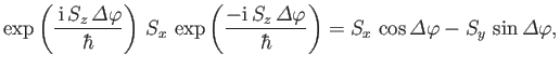
where use has been made of Equation (5.1).
Thus,
 |
(5.34) |
The second
proof is more general than the first, because it only makes use of the fundamental
commutation relation (5.1), and is, therefore, valid for systems with spin
angular momentum greater than one-half.
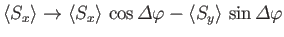
For a spin one-half system, both methods imply that
 |
(5.35) |
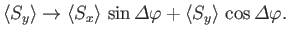
under the action of the rotation operator (5.24). It is straightforward to
show that
 |
(5.36) |
Furthermore,
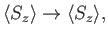 |
(5.37) |
because  commutes with the rotation operator. Equations (5.35)-(5.37)
demonstrate that
the operator (5.24) rotates the expectation value of
commutes with the rotation operator. Equations (5.35)-(5.37)
demonstrate that
the operator (5.24) rotates the expectation value of  through an
angle
about the
-axis. In fact, the expectation value
of the spin operator behaves like a classical vector under rotation. In other words,
through an
angle
about the
-axis. In fact, the expectation value
of the spin operator behaves like a classical vector under rotation. In other words,
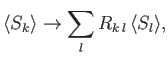 |
(5.38) |
where the  are the elements of the conventional rotation matrix
for the rotation in question [92]. (Here, and in the following,
are the elements of the conventional rotation matrix
for the rotation in question [92]. (Here, and in the following,  ,
,  , et cetera, are indices that run from 1 to 3, with 1 corresponding to the
  -axis, 2 to
the
-axis, 2 to
the  -axis, and so on.) It is clear, from our second derivation of
the result (5.35), that this property is not restricted to the spin operators of
a spin one-half system. In fact, we have effectively demonstrated that
-axis, and so on.) It is clear, from our second derivation of
the result (5.35), that this property is not restricted to the spin operators of
a spin one-half system. In fact, we have effectively demonstrated that
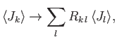 |
(5.39) |
where the  are the generators of rotation, satisfying the fundamental
commutation relation
are the generators of rotation, satisfying the fundamental
commutation relation
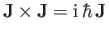 ,
and the rotation operator about the
th axis is written
,
and the rotation operator about the
th axis is written
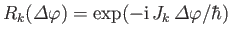 .
.
Consider the effect of the rotation operator (5.24) on the state ket (5.23).
It is easily seen that
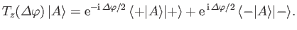 |
(5.40) |
Consider a rotation by  radians. We find that
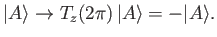 |
(5.41) |
Note that a ket rotated by
radians differs from the original ket by a
minus sign. In fact, a rotation by  radians is needed to transform a ket
into itself. The minus sign does not affect the expectation value of
, because
is sandwiched between
radians is needed to transform a ket
into itself. The minus sign does not affect the expectation value of
, because
is sandwiched between
 and
,
both of which change sign. Nevertheless, the minus sign does give rise to
observable consequences, as we shall see presently.
and
,
both of which change sign. Nevertheless, the minus sign does give rise to
observable consequences, as we shall see presently.
Next: Magnetic Moments
Up: Spin Angular Momentum
Previous: Wavefunction of Spin One-Half
Richard Fitzpatrick
2016-01-22
![$\displaystyle \equiv A + {\rm i} \,\lambda\, [G,A] + \left(\frac{{\rm i}^{\,2} \lambda^{\,2}}{2!}\right) [G, [G,A]]$](img1362.png)
![$\displaystyle \phantom{=}+ \left(\frac{{\rm i}^{\,3}\lambda^{\,3}}{3!}\right)[G, [G, [G,A]]]+\cdots,$](img1363.png)