Specific Heats of Solids
Consider a simple solid containing  atoms. Now, atoms in solids cannot
translate (unlike those in gases), but
are free to vibrate about their equilibrium positions.
Such vibrations are termed lattice vibrations, and can be thought of
as sound waves propagating
through the crystal lattice. Each atom is specified by three independent position
coordinates, and three corresponding momentum coordinates. Let us
only consider small-amplitude vibrations.
In this case, we can expand the potential energy of interaction between the atoms
to give an expression that is quadratic in the atomic displacements
from their equilibrium positions. It is always possible to perform a
normal mode analysis
of the oscillations. In effect, we can find
atoms. Now, atoms in solids cannot
translate (unlike those in gases), but
are free to vibrate about their equilibrium positions.
Such vibrations are termed lattice vibrations, and can be thought of
as sound waves propagating
through the crystal lattice. Each atom is specified by three independent position
coordinates, and three corresponding momentum coordinates. Let us
only consider small-amplitude vibrations.
In this case, we can expand the potential energy of interaction between the atoms
to give an expression that is quadratic in the atomic displacements
from their equilibrium positions. It is always possible to perform a
normal mode analysis
of the oscillations. In effect, we can find  independent modes of oscillation of the solid.
Each mode has its own particular oscillation frequency, and its own particular pattern
of atomic displacements.
Any general oscillation can be written as a linear combination of these
normal modes.
Let
independent modes of oscillation of the solid.
Each mode has its own particular oscillation frequency, and its own particular pattern
of atomic displacements.
Any general oscillation can be written as a linear combination of these
normal modes.
Let  be the (appropriately normalized) amplitude of the
  th normal mode,
and
th normal mode,
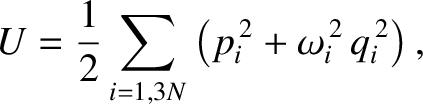
and  the corresponding momentum. In normal-mode coordinates, the internal energy of the lattice vibrations takes the
particularly simple form
the corresponding momentum. In normal-mode coordinates, the internal energy of the lattice vibrations takes the
particularly simple form
 |
(5.487) |
where  is the (angular) oscillation frequency of the th normal mode. It is
clear that, when expressed in normal-mode coordinates, the linearized lattice vibrations are equivalent to
independent harmonic oscillators. (Of course, each oscillator corresponds to a different normal
mode.)
is the (angular) oscillation frequency of the th normal mode. It is
clear that, when expressed in normal-mode coordinates, the linearized lattice vibrations are equivalent to
independent harmonic oscillators. (Of course, each oscillator corresponds to a different normal
mode.)
The typical value of is the (angular) frequency of a sound wave
propagating through the lattice. Sound wave frequencies are far lower than the
typical vibration frequencies of gaseous molecules. In the latter case, the mass involved in the
vibration is simply that of the molecule, whereas in the former case the mass involved is that
of very many atoms (because lattice vibrations are non-localized). The strength of
interatomic bonds in gaseous molecules is similar to those in solids, so we can use the estimate
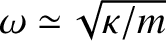 (
( is the force constant that measures the strength of
interatomic bonds, and
is the force constant that measures the strength of
interatomic bonds, and  is the mass involved in the oscillation) as proof that the typical
frequencies of lattice vibrations are very
much less than the vibration frequencies of simple molecules.
It follows, from
is the mass involved in the oscillation) as proof that the typical
frequencies of lattice vibrations are very
much less than the vibration frequencies of simple molecules.
It follows, from
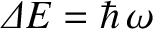 , that the quantum energy levels of lattice vibrations are
far more closely spaced than the vibrational energy levels of gaseous molecules. Thus, it is
likely (and is, indeed, the case) that lattice vibrations are not frozen out at room temperature,
but, instead, make their full classical contribution to the molar specific heat of the solid. (See Section 5.5.8.)
, that the quantum energy levels of lattice vibrations are
far more closely spaced than the vibrational energy levels of gaseous molecules. Thus, it is
likely (and is, indeed, the case) that lattice vibrations are not frozen out at room temperature,
but, instead, make their full classical contribution to the molar specific heat of the solid. (See Section 5.5.8.)
If the lattice vibrations behave classically then, according to the equipartition theorem (see Section 5.5.5),
each normal mode of oscillation has an associated mean energy  , in equilibrium at
temperature
, in equilibrium at
temperature  [
[
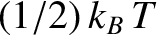 resides in the kinetic energy of the oscillation,
and
resides in the potential energy].
Thus, the internal energy of the solid is
resides in the kinetic energy of the oscillation,
and
resides in the potential energy].
Thus, the internal energy of the solid is
 |
(5.488) |
where
 .
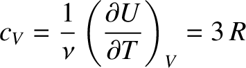
It follows that the molar heat capacity at constant volume is
.
It follows that the molar heat capacity at constant volume is
 |
(5.489) |
for solids. This gives a value of  joules/mole/degree. In fact, at room temperature, most
solids (in particular, metals)
have heat capacities that lie remarkably close to this value. This
fact was discovered
experimentally by Pierre Dulong and Alexis Petite at the beginning of the nineteenth century, and was used to
make some of the first
crude estimates of the molecular weights of solids. (If we know the molar heat capacity
of a substance
then we can easily work out how much of it corresponds to one mole, and
by weighing this amount, and then dividing the result by Avogadro's number,
we can then obtain an estimate of the molecular weight.)
joules/mole/degree. In fact, at room temperature, most
solids (in particular, metals)
have heat capacities that lie remarkably close to this value. This
fact was discovered
experimentally by Pierre Dulong and Alexis Petite at the beginning of the nineteenth century, and was used to
make some of the first
crude estimates of the molecular weights of solids. (If we know the molar heat capacity
of a substance
then we can easily work out how much of it corresponds to one mole, and
by weighing this amount, and then dividing the result by Avogadro's number,
we can then obtain an estimate of the molecular weight.)
Table 5.3 lists the experimental
molar heat
capacities,  , at constant pressure for various solids. The heat capacity at constant
volume is somewhat less than the constant pressure value, but not by much,
because solids
are fairly incompressible.
It can be seen that Dulong and Petite's law (i.e., that all solids have a molar heat capacities
close to joules/mole/degree) holds fairly well for metals.
However, the law fails badly for
diamond. This is not surprising. As is well known,
diamond is an extremely hard substance, so its interatomic bonds must be very strong, suggesting
that the force constant, , is large.
Diamond is also a fairly low-density substance, so the mass, , involved in
lattice vibrations is comparatively small. Both these facts suggest that the typical lattice vibration
frequency of diamond (
) is high. In fact, the spacing between
the different vibrational energy
levels (which scales like
, at constant pressure for various solids. The heat capacity at constant
volume is somewhat less than the constant pressure value, but not by much,
because solids
are fairly incompressible.
It can be seen that Dulong and Petite's law (i.e., that all solids have a molar heat capacities
close to joules/mole/degree) holds fairly well for metals.
However, the law fails badly for
diamond. This is not surprising. As is well known,
diamond is an extremely hard substance, so its interatomic bonds must be very strong, suggesting
that the force constant, , is large.
Diamond is also a fairly low-density substance, so the mass, , involved in
lattice vibrations is comparatively small. Both these facts suggest that the typical lattice vibration
frequency of diamond (
) is high. In fact, the spacing between
the different vibrational energy
levels (which scales like
 ) is sufficiently large in diamond for the vibrational
degrees of freedom
to be largely frozen out at room temperature. This accounts for the anomalously low
heat capacity of diamond in Table 5.3.
) is sufficiently large in diamond for the vibrational
degrees of freedom
to be largely frozen out at room temperature. This accounts for the anomalously low
heat capacity of diamond in Table 5.3.
Table: 5.3
Values of (joules/mole/degree) for some solids at
 K.
K.
| |
|
|
|
| Solid |
|
Solid |
|
| Copper |
24.5 |
Aluminium |
24.4 |
| Silver |
25.5 |
Tin (white) |
26.4 |
| Lead |
26.4 |
Sulphur (rhombic) |
22.4 |
| Zinc |
25.4 |
Carbon (diamond) |
6.1 |
|
Dulong and Petite's law is essentially a high-temperature limit. We can make
a crude model of the behavior of  at low temperatures by assuming that all of the normal
modes oscillate at the same frequency,
at low temperatures by assuming that all of the normal
modes oscillate at the same frequency,  (say). This approximation was first employed by
Einstein in a paper published in 1907. According to Equation (5.487),
the solid acts like a set
of independent oscillators which, making use of
Einstein's approximation, all vibrate at the same frequency.
We can use the quantum mechanical result (5.390) for the mean energy of a single
oscillator to write the internal energy
of the solid in the form
(say). This approximation was first employed by
Einstein in a paper published in 1907. According to Equation (5.487),
the solid acts like a set
of independent oscillators which, making use of
Einstein's approximation, all vibrate at the same frequency.
We can use the quantum mechanical result (5.390) for the mean energy of a single
oscillator to write the internal energy
of the solid in the form
![$\displaystyle U = 3\,N \left[\frac{1}{2} +
\frac{1}{\exp(\hbar\,\omega/k_B\,T) - 1} \right]\hbar\,\omega,$](img4387.png) |
(5.490) |
giving
![$\displaystyle c_V \frac{1}{\nu}\left(\frac{\partial U}{\partial T}\right)_V= 3\...
...c{\theta_E}{T}\right)^2 \frac{\exp(\theta_E / T)}
{[\exp(\theta_E/T) - 1]^{2}}.$](img4388.png) |
(5.491) |
Here,
 |
(5.492) |
is termed the Einstein temperature. If the temperature is sufficiently
high that
 then the previous expression reduces to
 , after expansion of the exponential functions. Thus, the law of Dulong and
Petite is recovered for temperatures significantly in excess of the Einstein temperature.
On the other hand, if the temperature is sufficiently
low that
, after expansion of the exponential functions. Thus, the law of Dulong and
Petite is recovered for temperatures significantly in excess of the Einstein temperature.
On the other hand, if the temperature is sufficiently
low that
 then the
exponential factors appearing in Equation (5.491) become very much larger than unity, giving
then the
exponential factors appearing in Equation (5.491) become very much larger than unity, giving
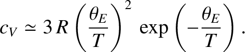 |
(5.493) |
So, in this simple model, the specific heat approaches zero exponentially as
 .
.
In reality, the specific heats of solids do not approach zero quite as quickly as
suggested by Einstein's model when
. The experimentally observed low-temperature
behavior is more like
 . The reason for this discrepancy is the crude
approximation
that all normal modes have the same frequency. In fact, long-wavelength modes have lower frequencies
than short-wavelength modes, so the former are much harder to freeze out than the latter
(because the spacing between quantum energy levels,
, is smaller in the former case).
The molar
heat capacity does not decrease with temperature as rapidly as suggested by Einstein's model
because these long-wavelength modes are able to make a significant contribution
to the heat capacity, even at very low
temperatures. A more realistic model of lattice vibrations was developed by
Peter Debye in 1912.
In the Debye model, the frequencies of the normal modes of vibration are estimated by treating
the solid as an isotropic continuous medium. This approach is reasonable because the only modes
that really matter at low temperatures are the long-wavelength modes; more explicitly, those whose
wavelengths greatly exceed the interatomic spacing. It is plausible that these modes are not
particularly
sensitive to the discrete nature of the solid. In other words, they are not sensitive to the fact that the solid is made up of atoms,
rather than being continuous.
. The reason for this discrepancy is the crude
approximation
that all normal modes have the same frequency. In fact, long-wavelength modes have lower frequencies
than short-wavelength modes, so the former are much harder to freeze out than the latter
(because the spacing between quantum energy levels,
, is smaller in the former case).
The molar
heat capacity does not decrease with temperature as rapidly as suggested by Einstein's model
because these long-wavelength modes are able to make a significant contribution
to the heat capacity, even at very low
temperatures. A more realistic model of lattice vibrations was developed by
Peter Debye in 1912.
In the Debye model, the frequencies of the normal modes of vibration are estimated by treating
the solid as an isotropic continuous medium. This approach is reasonable because the only modes
that really matter at low temperatures are the long-wavelength modes; more explicitly, those whose
wavelengths greatly exceed the interatomic spacing. It is plausible that these modes are not
particularly
sensitive to the discrete nature of the solid. In other words, they are not sensitive to the fact that the solid is made up of atoms,
rather than being continuous.
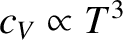
According to Equation (5.461), the density of sound wave states in a continuous solid is
 |
(5.494) |
where  is the average sound speed.
The Debye approach consists in approximating the actual density of sound wave states,
is the average sound speed.
The Debye approach consists in approximating the actual density of sound wave states,
 , by the density in a continuous medium,
 , not
only at low frequencies (long wavelengths) where these should be nearly the same, but
also at high frequencies where they may differ substantially. Suppose that we are
dealing with a solid consisting of atoms. We know that there are
only independent normal modes. It follows that we must cut off the
density of states above some critical frequency,
, not
only at low frequencies (long wavelengths) where these should be nearly the same, but
also at high frequencies where they may differ substantially. Suppose that we are
dealing with a solid consisting of atoms. We know that there are
only independent normal modes. It follows that we must cut off the
density of states above some critical frequency,  (say), otherwise we
will have too many modes. Thus, in the Debye approximation, the density
of normal modes takes the form
(say), otherwise we
will have too many modes. Thus, in the Debye approximation, the density
of normal modes takes the form
![\begin{displaymath}\rho_D(\omega) = \left\{
\begin{array}{lll}\rho_c(\omega) &\m...
...eq \omega_D\\ [0.5ex]
0& & \omega>\omega_D
\end{array}\right. .\end{displaymath}](img4400.png) |
(5.495) |
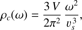
Here, is termed the Debye frequency, and is chosen such that
the total number of normal modes is :
 |
(5.496) |
Substituting Equation (5.494) into the previous formula yields
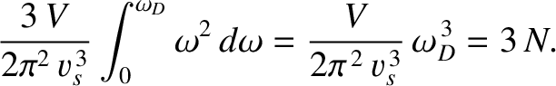 |
(5.497) |
This implies that
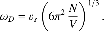 |
(5.498) |
Thus, the Debye frequency depends only on the sound speed in the solid, and the number
of atoms per unit volume. The wavelength corresponding to the Debye frequency
is
 , which is clearly on the order of the interatomic spacing,
 .
It follows that the cut-off of normal modes whose frequencies exceed the Debye frequency
is equivalent to a cut-off of normal modes whose wavelengths are less than the interatomic
spacing. Of course, it makes physical sense that such modes should be absent.
.
It follows that the cut-off of normal modes whose frequencies exceed the Debye frequency
is equivalent to a cut-off of normal modes whose wavelengths are less than the interatomic
spacing. Of course, it makes physical sense that such modes should be absent.
We can use the quantum-mechanical expression for the
mean energy of a single oscillator, Equation (5.390), to calculate the internal energy associated with lattice vibrations in the Debye approximation. We obtain
![$\displaystyle U = \int_0^\infty \rho_D(\omega)
\left[\frac{1}{2} + \frac{1}{\exp(\hbar\, \omega/k_B\,T)-1}\right]\hbar\,\omega\,d\omega.$](img4406.png) |
(5.499) |
Hence, the molar heat capacity takes the form
![$\displaystyle c_V =\frac{1}{\nu}\left(\frac{\partial U}{\partial T}\right)_V
= ...
...,\omega}
{[\exp(\hbar\,\omega/k_B\,T)-1]^{\,2}}\right\}
\hbar\,\omega\,d\omega.$](img4407.png) |
(5.500) |
Making use of Equations (5.494) and (5.495), we find that
![$\displaystyle c_V = \frac{k_B}{\nu}\int_0^{\omega_D} \frac{\exp(\hbar\,\omega/k...
...\omega/k_B\,T)-1]^{2}}\,
\frac{3 \,V}{2\pi^2 \,v_s^{\,3}}\,\omega^{2}\,d\omega,$](img4408.png) |
(5.501) |
giving
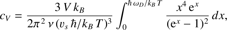 |
(5.502) |
in terms of the dimensionless variable
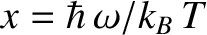 .
According to Equation (5.498), the volume can be written
.
According to Equation (5.498), the volume can be written
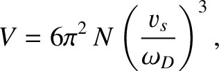 |
(5.503) |
so the heat capacity reduces to
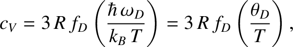 |
(5.504) |
where the Debye function is defined
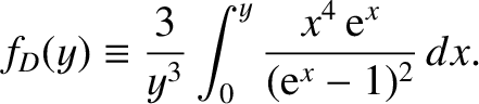 |
(5.505) |
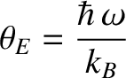
We have also defined the Debye temperature,  , as
, as
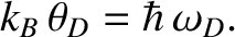 |
(5.506) |
Consider the asymptotic limit in which
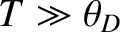 . For small
  , we can approximate
 as
as  in the integrand of Equation (5.505), so that
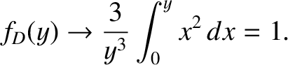 |
(5.507) |
Thus, if the temperature greatly exceeds the Debye temperature then we recover the law of
Dulong and Petite that
. Consider, now, the
asymptotic limit in which
 . For large ,
 |
(5.508) |
The latter integral can be looked up in standard reference books on integrals. Thus, in the low-temperature limit,
 |
(5.509) |
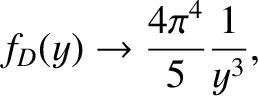
which yields
 |
(5.510) |
in the limit
, Note that varies with temperature as  , in accordance with experimental
observation.
, in accordance with experimental
observation.
Table 5.4:
Comparison of Debye temperatures (in degrees kelvin) obtained from the
low temperature behavior of the heat capacity with those calculated from the
sound speed.
| Solid |
(low temperature) |
(sound speed) |
| Na Cl |
308 |
320 |
| K Cl |
230 |
246 |
| Ag |
225 |
216 |
| Zn |
308 |
305 |
|
The fact that goes like at low temperatures is quite well verified experimentally,
although it is sometimes necessary to go to temperatures as low as
 to obtain
this asymptotic behavior. Theoretically, should be calculable from
Equation (5.498)
in terms of the sound speed in the solid, and the molar volume. Table 5.4 shows a
comparison of Debye temperatures evaluated by this means with temperatures obtained
empirically by fitting the law (5.510) to the low-temperature variation of the
heat capacity. It can be seen that there is fairly good agreement between the theoretical and
empirical Debye temperatures. This suggests that the Debye theory affords a good, though not
perfect, representation of the behavior of in solids over the entire temperature range.
to obtain
this asymptotic behavior. Theoretically, should be calculable from
Equation (5.498)
in terms of the sound speed in the solid, and the molar volume. Table 5.4 shows a
comparison of Debye temperatures evaluated by this means with temperatures obtained
empirically by fitting the law (5.510) to the low-temperature variation of the
heat capacity. It can be seen that there is fairly good agreement between the theoretical and
empirical Debye temperatures. This suggests that the Debye theory affords a good, though not
perfect, representation of the behavior of in solids over the entire temperature range.
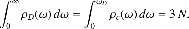
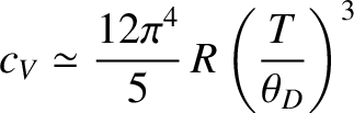
Figure: 5.9
The molar heat capacity of various solids. The solid
curve shows the prediction of Debye theory. The dotted curve shows the prediction of Einstein theory (assuming that
 ).
).
|
|
Finally, Figure 5.9 shows the actual temperature variation of the molar heat capacities
of various solids, as well as that predicted by Debye's theory. The prediction of Einstein's theory
is also shown, for the sake of comparison.
![\includegraphics[width=0.85\textwidth]{Chapter06/debye.eps}](img4426.png)