Conduction Electrons in Metal

The conduction electrons in a metal are non-localized (i.e., they are not tied to any particular atoms). In conventional metals, each atom contributes a fixed number of such electrons (corresponding to its valency). To a first approximation, it is possible to neglect the mutual interaction of the conduction electrons, because this interaction is largely shielded out by the stationary ions. The conduction electrons can, therefore, be treated as an ideal gas. However, the number density of such electrons in a metal far exceeds the number density of molecules in a conventional gas.

Electrons are subject to the Pauli exclusion principle, according to which a given electron state can either be unoccupied, or singly occupied. (See Section 4.4.3.) The so-called Fermi energy is the energy at which electrons are available without doing work. Thus, an electron state of energy $\epsilon$ has an available free energy 0 when it is unoccupied, and an available free energy $\epsilon-\epsilon_F$ when it is occupied. According to the Boltzmann distribution (see Section 5.4.7), the relative probabilities of unoccupied and occupied states are thus $P(0)=1$ and $P(1)= \exp[-(\epsilon-\epsilon_F)/(k_B\,T)]$, respectively, where $T$ is the temperature. (See Section 5.4.7.) Thus, the mean occupancy number of the state is

$$F(\epsilon) = \frac{0\times P(0)+ 1\times P(1)}{P(0)+P(1)},$$ (5.511)

which reduces to

$$F(\epsilon) = \frac{1}{\exp[(\epsilon-\epsilon_F)/(k_B\,T)]+1}.$$ (5.512)

Here, $F(\epsilon)$ is termed the Fermi function.

Let us investigate the behavior of the Fermi function as $\epsilon$ varies. Here, the energy is measured from its lowest possible value $\epsilon=0$. The Fermi energy for conduction electrons in a metal is such that $\epsilon_F\gg k_B\,T$. In this limit, if $0<\epsilon\ll \epsilon_F$ then $(\epsilon-\epsilon_F)/(k_B\,T)\ll -1$, so that $F(\epsilon)\simeq 1$. On the other hand, if $\epsilon\gg \epsilon_F$ then $(\epsilon-\epsilon_F)/(k_B\,T)\gg 1$, so that $F(\epsilon)\simeq \exp[-(\epsilon-\mu)/(k_B\,T)]$ falls off exponentially with increasing $\epsilon$. Note that $F=1/2$ when $\epsilon=\epsilon_F$. The transition region in which $F$ goes from a value close to unity to a value close to zero corresponds to an energy interval of order $k_B\,T$, centered on $\epsilon=\epsilon_F$. In fact, $F=3/4$ when $\epsilon=\epsilon_F-(\ln 3)\,k_B\,T$, and $F=1/4$ when $\epsilon=\epsilon_F+(\ln 3)\,k_B\,T$. The behavior of the Fermi function is illustrated in Figure 5.10.

Figure 5.10: The Fermi function.

In the limit as $T\rightarrow 0$, the transition region becomes infinitesimally narrow. In this case, $F=1$ for $\epsilon\leq \epsilon_F$, and $F=0$ for $\epsilon>\epsilon_F$, as illustrated in Figure 5.10. This is an obvious result, because when $T=0$ the conduction electrons attain their lowest energy, or ground-state, configuration. Because the Pauli exclusion principle requires that there be no more than one electron per single-particle quantum state, the lowest energy configuration is obtained by piling electrons into the lowest available unoccupied states, until all of the electrons are used up. Thus, the last electron added to the pile has a quite considerable energy, $\epsilon=\epsilon_F$, because all of the lower energy states are already occupied. Clearly, the exclusion principle implies that free electrons in a metal possess a large mean energy, even at a temperature of absolute zero.

We can calculate the Fermi energy by equating the number of occupied electron states to the total number of electrons in the metal, $N_e$. In other words,

$$\int_0^\infty F(\epsilon)\,\rho(\epsilon)\,d\epsilon = N_e,$$ (5.513)

where $\rho(\epsilon)$ is the density of electron states specified in Equation (5.466). Assuming that $\epsilon_F\gg k_B\,T$, we can make the approximation

$$F(\epsilon) \simeq \left\{\begin{array}{lll} 1&~~~&0\leq\epsilon\leq \epsilon_F\\ [0.5ex] 0&&\epsilon>\epsilon_F\end{array}\right..$$ (5.514)

Thus, making use of Equation (5.466), we obtain

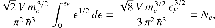$$\frac{\sqrt{2}\,V\,m_e^{\,3/2}}{\pi^2\,\hbar^3} \int_0^{\epsilon_... ...\frac{\sqrt{8}\,V\,m_e^{\,3/2}\,\epsilon_F^{\,3/2}}{3\,\pi^2\,\hbar^{3}} = N_e,$$ (5.515)

which can be rearranged to give

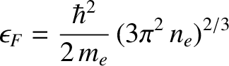$$\epsilon_F = \frac{\hbar^2}{2\,m_e}\,(3\pi^2\,n_e)^{2/3}$$ (5.516)

where $n_e=N_e/V$ is the number density of conduction electrons. The mean electron energy is

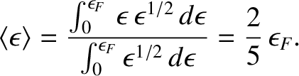$$\langle \epsilon\rangle = \frac{\int_0^{\epsilon_F}\,\epsilon\,\e... ...psilon}{\int_0^{\epsilon_F}\epsilon^{1/2}\,d\epsilon} =\frac{2}{5}\,\epsilon_F.$$ (5.517)

(See Section 4.4.3.)

Copper at room temperature has a number density of conduction electrons of $n_e=8.4\times 10^{28}\,{\rm m}^{-3}$. According to Equation (5.516), the corresponding Fermi energy is

$$\epsilon_F = 7.0\,{\rm eV}.$$ (5.518)

The associated Fermi temperature is

$$\theta_F= \frac{\epsilon_F}{k_B} = 8.1\times 10^4\,{\rm K}.$$ (5.519)

Thus, at room temperature, $T=288$ K, we obtain

$$\frac{k_B\,T}{\epsilon_F}=\frac{\theta_F}{T} \simeq \frac{1}{280},$$ (5.520)

which confirms that $\epsilon_F\gg k_B\,T$ for conduction electrons in a metal.

Figure 5.11: Approximate Fermi function.

Let us crudely approximate the Fermi function at finite temperature in the fashion shown in Figure 5.11. As can be seen from the figure, the proportion of thermally excited electrons is the ratio of the area of a triangle of height $1/2$ and base $2\,k_B\,T$ to that of a rectangle of height 1 and base $\epsilon_F$. In other words,

$$\frac{(1/2)\,(1/2)\,(2\,k_B\,T)}{\epsilon_F} = \frac{k_B\,T}{2\,\epsilon_F}.$$ (5.521)

Now, the centroid of a right-angled triangle is $1/3$ rd of the distance along its base from the right-angle. Thus, the mean energy of the excited electrons increases by

$$2\,\frac{1}{3}\,2\,k_B\,T= \frac{4}{3}\,k_B\,T.$$ (5.522)

Hence, the thermal energy per conduction electron is

$$\left(\frac{k_B\,T}{2\,\epsilon_F}\right)\left(\frac{4}{3}\,k_B\,T\right) = \frac{2\,k_B^{\,2}\,T^2}{3\,\epsilon_F},$$ (5.523)

which implies that the internal energy (i.e., the difference between the energy at a finite temperature and the energy at absolute zero) of the conduction electrons is

$$U \simeq N_e\,\frac{2\,k_B^{\,2}\,T^2}{3\,\epsilon_F} = \frac{2\,\nu\,R\,k_B\,T^2}{3\,\epsilon_F},$$ (5.524)

where $\nu$ is the number of moles of electrons. Finally, the molar specific heat of the electrons at constant volume is

$$c_V \simeq \frac{1}{\nu}\,\left(\frac{\partial U}{\partial T}\right)_V = \frac{4\,R\,k_B\,T}{3\,\epsilon_F},$$ (5.525)

which can also be written

$$c_V \simeq \left(\frac{3}{2}\,R\right)\left(\frac{8}{9}\,\frac{T}{\theta_F}\right).$$ (5.526)

The exact result is

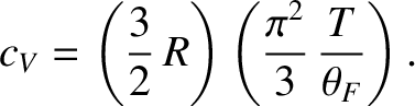$$c_V = \left(\frac{3}{2}\,R\right)\left(\frac{\pi^2}{3}\,\frac{T}{\theta_F}\right).$$ (5.527)

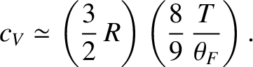
Thus, we conclude that the contribution of the conduction electrons to the molar specific heat capacity of a metal is proportional to the temperature. However, this contribution is much less that the classical contribution, $(3/2)\,R$, predicted by the equipartition theorem (see Section 5.5.5), given that each conduction electron possesses three translational degrees of freedom. This is the case because the conduction electrons in a metal are highly degenerate. (See Section 4.4.3.) In fact, Equations (5.520) and (5.527) imply that the contribution of the conduction electrons to the molar specific heat of copper at room temperature is a factor 85 times smaller than the classical contribution.

Using the superscript $e$ to denote the electronic specific heat due to conduction electrons, the molar specific heat of such electrons can be written

$$c_V^{(e)} = \gamma\,T,$$ (5.528)

where $\gamma$ is a (positive) constant of proportionality. At room temperature, $c_V^{(e)}$ is completely masked by the much larger specific heat, $c_V^{(L)}$, due to lattice vibrations. However, at very low temperatures, $c_V^{(L)}=A\,T^{3}$, where $A$ is a (positive) constant of proportionality. (See Section 5.6.5.) Clearly, at low temperatures, $c_V^{(L)}=A\,T^{3}$ approaches zero far more rapidly than the electronic specific heat, as $T$ is reduced. Hence, it should be possible to measure the electronic contribution to the molar specific heat at low temperatures.

Figure: 5.12 The low-temperature heat capacity of potassium, plotted as $c_V/T$ versus $T^{2}$. The straight-line shows the fit $c_V/T = 2.08+2.57\,T^{2}$.

The total molar specific heat of a metal at low temperatures takes the form

$$c_V = c_V^{(e)} + c_V^{(L)} = \gamma\,T + A\,T^{3}.$$ (5.529)

Hence,

$$\frac{c_V}{T} = \gamma + A\,T^{2}.$$ (5.530)

It follows that a plot of $c_V/T$ versus $T^{2}$ should yield a straight-line whose intercept on the vertical axis gives the coefficient $\gamma$. Figure 5.12 shows such a plot. The fact that a good straight-line, with a non-zero intercept, is obtained verifies that the temperature dependence of the heat capacity predicted by Equation (5.529) is indeed correct.