Equipartition Theorem
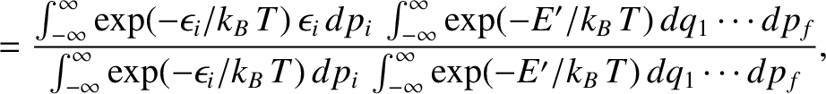
The internal energy of a monatomic ideal gas containing  atoms is
 . (See Section 5.2.3.)
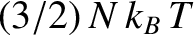
This implies that each atom possess, on average,
. (See Section 5.2.3.)
This implies that each atom possess, on average,
 units of energy.
Monatomic particles have only three translational degrees
of freedom, corresponding to
their motion in three dimensions. They possess no internal
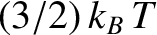
rotational or vibrational degrees of freedom. Thus, the mean energy per degree of
freedom in a monatomic ideal gas is
units of energy.
Monatomic particles have only three translational degrees
of freedom, corresponding to
their motion in three dimensions. They possess no internal
rotational or vibrational degrees of freedom. Thus, the mean energy per degree of
freedom in a monatomic ideal gas is
 . In fact,
this is a special case of a more general result. Let us now try to prove this result.
. In fact,
this is a special case of a more general result. Let us now try to prove this result.
Suppose that the energy of a
system is determined by  coordinates,
  ,
and corresponding momenta,
,
and corresponding momenta,  , so that
 |
(5.366) |
Suppose further that:
- The total energy splits additively into the form
 |
(5.367) |
where
 involves only one variable,
  , and the remaining part,
 , does not depend on .
- The function
is quadratic in , so that
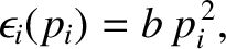 |
(5.368) |
where  is a constant.
The most common situation in which the previous assumptions are valid is where
is a momentum. This is because the kinetic energy is usually a quadratic
function of each momentum component, whereas the potential energy does not
involve the momenta at all. However, if a coordinate,  , were to satisfy
assumptions 1 and 2 then the theorem that we are about to establish would hold just
as well.
, were to satisfy
assumptions 1 and 2 then the theorem that we are about to establish would hold just
as well.
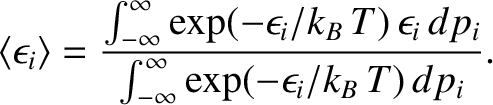
What is the mean value of
in thermal equilibrium if conditions
1 and 2 are satisfied? If the system is in equilibrium at absolute temperature
 then it is distributed according to the Boltzmann probability
distribution. (See Section 5.4.7.) In the classical approximation,
the mean value of
is expressed in terms of
integrals over all phase-space (see Section 5.4.4):
then it is distributed according to the Boltzmann probability
distribution. (See Section 5.4.7.) In the classical approximation,
the mean value of
is expressed in terms of
integrals over all phase-space (see Section 5.4.4):
![$\displaystyle \langle\epsilon_i\rangle = \frac{
\int_{-\infty}^{\infty} \exp[-E...
...
{\int_{-\infty}^{\infty} \exp[- E(q_1,\cdots, p_f)/k_B\,T]\,
dq_1\cdots dp_f}.$](img4127.png) |
(5.369) |
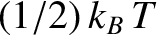
Condition 1 gives
where use has been made of the multiplicative property of the exponential function,
and where the final integrals in both the numerator and denominator extend over
all variables,
and , except for . These integrals are equal and, thus, cancel.
Hence,
 |
(5.371) |
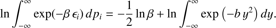
This expression can be simplified further because, writing
 ,
,
![$\displaystyle \int_{-\infty}^\infty
\exp(-\beta \,\epsilon_i)\,\epsilon_i\, dp_...
...ial \beta}
\left[\int_{-\infty}^\infty \exp(-\beta \,\epsilon_i)\, dp_i\right],$](img4133.png) |
(5.372) |
so
![$\displaystyle \langle\epsilon_i\rangle = - \frac{\partial}{\partial\beta}
\ln\left[\int_{-\infty}^\infty \exp(-\beta \,\epsilon_i)\,
dp_i\right].$](img4134.png) |
(5.373) |
According to condition 2,
 |
(5.374) |
where
 . Thus,
 |
(5.375) |
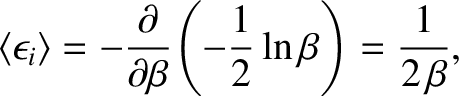
Note that the integral on the right-hand side is independent of  . It follows
from Equation (5.373) that
. It follows
from Equation (5.373) that
 |
(5.376) |
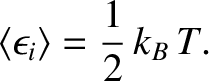
giving
 |
(5.377) |
This result is known as the equipartition theorem.
It states that the mean value of every independent
quadratic term in the energy is equal to
. If all terms in the energy are quadratic
then the mean energy is spread equally over all degrees of freedom. (Hence, the
name “equipartition.”)

![$\displaystyle =\frac{
\int_{-\infty}^{\infty} \exp[-(\epsilon_i + E')/k_B\,T]\,...
...p_f}
{\int_{-\infty}^{\infty} \exp[-(\epsilon_i + E')/k_B\,T]\,dq_1\cdots dp_f}$](img4129.png)