Gaussian Probability Distribution
Consider a very large number of observations,  , made on a system
with two possible outcomes. (See Sections 5.1.2 and 5.1.4.)
Suppose that the probability of outcome
, made on a system
with two possible outcomes. (See Sections 5.1.2 and 5.1.4.)
Suppose that the probability of outcome  is sufficiently large that
the average number of occurrences after
is sufficiently large that
the average number of occurrences after  observations is much greater than unity; that is,
 |
(5.61) |
In this limit, the standard deviation of  is also much greater than unity,
 |
(5.62) |
implying that there are very many probable values of scattered about the
mean value,
 .
This suggests that the probability of obtaining occurrences
of outcome
does not change significantly in going from one possible value of
to an adjacent value. In other words,
.
This suggests that the probability of obtaining occurrences
of outcome
does not change significantly in going from one possible value of
to an adjacent value. In other words,
 |
(5.63) |
In this situation, it is useful to regard the probability as a smooth
function of . Let now be a continuous variable that is
interpreted as the number of occurrences of outcome (after
observations) whenever it takes
on a positive integer value. The probability that lies between
and  is defined
 |
(5.64) |
where  is a probability density (see Section 5.1.6), and is independent
of
is a probability density (see Section 5.1.6), and is independent
of  . The probability can be written in this form because
 can always be expanded as a Taylor series in , and must go
to zero as
can always be expanded as a Taylor series in , and must go
to zero as
 .
We can write
.
We can write
 |
(5.65) |
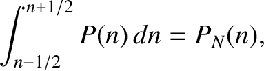
which is equivalent to smearing out the discrete probability  over the range
  . Given Equations (5.27) and (5.63), the previous relation
can be approximated as
. Given Equations (5.27) and (5.63), the previous relation
can be approximated as
 |
(5.66) |
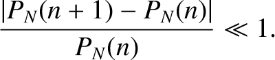
For large , the relative width of the probability distribution function
is small; that is,
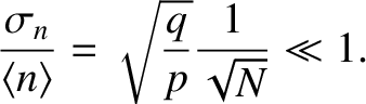 |
(5.67) |
This suggests that is strongly peaked around the mean value,
. Suppose that  attains
its maximum value at
attains
its maximum value at
 (where we expect
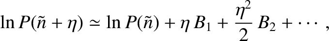
 ). Let us Taylor expand around
.
Note that we are expanding the slowly-varying function ,
rather than the rapidly-varying function ,
because the Taylor expansion of
does not converge sufficiently rapidly in the
vicinity of
to be useful.
We can write
). Let us Taylor expand around
.
Note that we are expanding the slowly-varying function ,
rather than the rapidly-varying function ,
because the Taylor expansion of
does not converge sufficiently rapidly in the
vicinity of
to be useful.
We can write
 |
(5.68) |
where
 |
(5.69) |
By definition,
if
corresponds to the maximum
value of .
It follows from Equation (5.66) that
 |
(5.72) |
If is a large integer, such that  , then
  is almost a
continuous function of , because changes by only a relatively
small amount when is incremented by unity.
Hence,
is almost a
continuous function of , because changes by only a relatively
small amount when is incremented by unity.
Hence,
![$\displaystyle \frac{d\ln n!}{dn} \simeq \frac{\ln\,(n+1)!-\ln n!}{1} =
\ln \left[\frac{(n+1)!}{n!}\right] = \ln\,(n+1),$](img3507.png) |
(5.73) |
giving
 |
(5.74) |
for . The integral of this relation
 |
(5.75) |
valid for , is called Stirling's approximation, after James Stirling, who first obtained it in 1730.
According to Equations (5.69), (5.72), and (5.74),
 |
(5.76) |
Hence, if  then
then
 |
(5.77) |
giving
 |
(5.78) |
because  . [See Equations (5.9) and (5.32).] Thus, the maximum of occurs exactly
at the mean value of .
. [See Equations (5.9) and (5.32).] Thus, the maximum of occurs exactly
at the mean value of .
Further differentiation of Equation (5.76) yields [see Equation (5.69)]
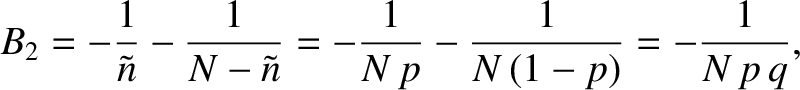 |
(5.79) |
because . Note that  , as required. According to Equation (5.62), the previous relation
can also be written
, as required. According to Equation (5.62), the previous relation
can also be written
 |
(5.80) |
It follows, from the previous analysis, that the Taylor expansion of can be written
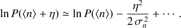 |
(5.81) |
Taking the exponential of both sides, we obtain
![$\displaystyle P(n)\simeq P(\langle n\rangle)\exp\left[-
\frac{(n-\langle n\rangle)^{2}}{2\,\sigma_n^{\,2}}\right].$](img3518.png) |
(5.82) |
The constant
 is most conveniently
fixed by making use
of the normalization condition,
is most conveniently
fixed by making use
of the normalization condition,
 |
(5.83) |
for a continuous distribution function. [See Equation (5.54). Note that cannot take a negative value.] Because we only expect
to be significant when
lies in the relatively narrow range
 , the limits of integration in the previous
expression can be replaced by
, the limits of integration in the previous
expression can be replaced by
 with negligible error.
Thus,
with negligible error.
Thus,
 |
(5.84) |
As is well known,
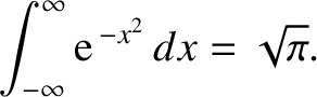 |
(5.85) |
It follows from the normalization condition (5.84) that
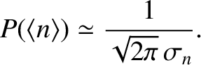 |
(5.86) |
Finally, we obtain
![$\displaystyle P(n) \simeq \frac{1}{\sqrt{2\pi} \,\sigma_n}\,
\exp\left[-\frac{(n-\langle n\rangle)^{2}}{2\,\sigma_n^{\,2}}\right].$](img3526.png) |
(5.87) |
This is probability distribution is known as Gaussian probability distribution, after the
Carl F. Gauss, who discovered in 1809 it while
investigating the distribution of errors in measurements. The Gaussian
distribution is only valid in the limits and
 .
According to this distribution, at one standard deviation away from the mean value—that is
.
According to this distribution, at one standard deviation away from the mean value—that is
 —the probability density is
about 61% of its peak value. At two standard deviations away from the mean
value, the probability density is about 13.5% of its peak value.
Finally,
at three standard deviations away from the mean value, the probability
density is only about 1% of its peak value. We conclude
that there is
very little chance that lies more than about three standard deviations
away from its mean value. In other words, is almost certain to lie in the
relatively narrow range
—the probability density is
about 61% of its peak value. At two standard deviations away from the mean
value, the probability density is about 13.5% of its peak value.
Finally,
at three standard deviations away from the mean value, the probability
density is only about 1% of its peak value. We conclude
that there is
very little chance that lies more than about three standard deviations
away from its mean value. In other words, is almost certain to lie in the
relatively narrow range
 .
.
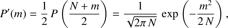
Consider the drunken walk discussed at the end of Section 5.1.2.
Suppose that the drunken man is equally likely to take a step to the right as to take a step
to the left. In other words,  . Thus, according to Equations (5.32) and (5.41),
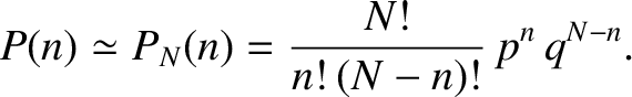
Equations (5.18) and (5.19) state that the probability of the drunken man taking  net steps
to the right after total steps is
net steps
to the right after total steps is
 |
(5.90) |
where
 |
(5.91) |
In the limit of very many steps, we can treat and as continuous variables. Let
 be the probability that lies between and
  . Likewise,
let
. Likewise,
let  be the probability that lies between and .
It follows that
be the probability that lies between and .
It follows that
 |
(5.92) |
where and satisfy Equation (5.91). Hence,
 |
(5.93) |
where use has been made of Equations (5.87), (5.88), (5.89), and (5.91).
Suppose that each step is of length  , and that the man takes
  steps per second. It follows that
the man's displacement from his starting point is
steps per second. It follows that
the man's displacement from his starting point is  . Moreover,
  . Let
. Let
 be the probability that the man's displacement from his starting point after
  seconds lies
between
seconds lies
between  and
and  . We have
 , which implies that
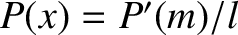 .
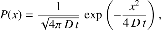
Hence, we obtain
.
Hence, we obtain
 |
(5.94) |
where
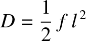 |
(5.95) |
is the diffusivity. It is easily demonstrated that
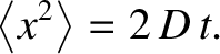 |
(5.96) |
Thus, it is evident from the analysis of Section 5.1.5 that the probability density distribution (5.94) corresponds to
that of a random walk in one dimension. Equation (5.94) can also be thought of as describing the diffusion
of probability density along the -axis. (See Section 5.3.9.)