Application to Binomial Probability Distribution
Let us now apply what we have just learned about the mean, variance, and
standard deviation of a general probability distribution
to the specific case of the
binomial probability distribution. Recall, from Section 5.1.2,
that if a simple system has just two possible outcomes,
denoted  and
and  , with
respective probabilities
, with
respective probabilities  and
and  ,
then the probability of obtaining
,
then the probability of obtaining  occurrences of outcome in
  observations is
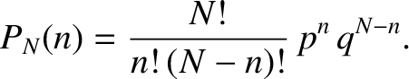 |
(5.27) |
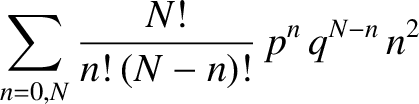
Thus, making use of Equation (5.21), the mean number of occurrences of outcome in observations
is given by
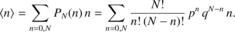 |
(5.28) |
We can see that if the
final factor
were absent on the right-hand side of the previous expression then it would just reduce to the binomial expansion, which we
know how to sum. [See Equation (5.16).] We can take advantage of this fact using a rather elegant
mathematical sleight of hand. Observe that because
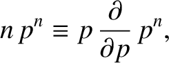 |
(5.29) |
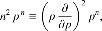
the previous summation can be rewritten as
![$\displaystyle \sum_{n=0,N}\frac{N!}{n!\,(N-n)!}\,p^{n}\,q^{\,N-n}\, n
\equiv p\...
...{\partial p}\!\left[\sum_{n=0,N}
\frac{N!}{n!\,(N-n)!}\,p^{n}\,q^{N-n}
\right].$](img3427.png) |
(5.30) |
The term in square brackets is now the familiar binomial expansion, and
can be written more succinctly as 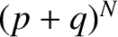 .
Thus,
.
Thus,
 |
(5.31) |
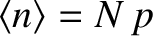
However, 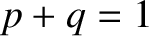 for the case in hand [see Equation (5.9)], so
 |
(5.32) |
In fact, we could have guessed the previous result.
By definition, the probability, , is the number of occurrences of the
outcome divided by the number of observations, in the limit as the number
of observations goes to infinity:
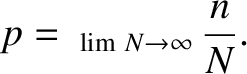 |
(5.33) |
[See Equation (5.1).]
If we think carefully, however,
we can appreciate that taking the limit as the number
of observations goes to infinity is equivalent to taking the mean value,
so that
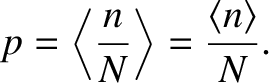 |
(5.34) |
But, this is just a simple rearrangement of Equation (5.32).
Let us now calculate the variance of . Recall, from Equation (5.25), that
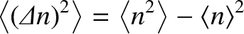 |
(5.35) |
We already know
 ,
so we just need to calculate
,
so we just need to calculate
 .
This average is written
.
This average is written
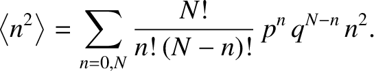 |
(5.36) |
The sum can be evaluated using a simple extension of the mathematical trick that
we used previously to evaluate
. Because
 |
(5.37) |
we can write
Using , we obtain
because
 . [See Equation (5.32).] It follows that the variance
of is given by
. [See Equation (5.32).] It follows that the variance
of is given by
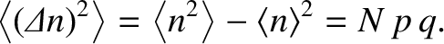 |
(5.40) |
The standard deviation of is the square root of the variance [see Equation (5.26)], so that
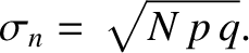 |
(5.41) |
Now, the standard deviation is essentially the width of the range of probable values over which
is distributed around its mean value,
. The relative width of the
distribution is characterized by
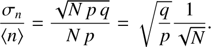 |
(5.42) |
It is clear, from the previous formula, that the relative width decreases with increasing like
 . So, the greater the number of observations, the
more likely it is that an observation of will yield a result
that is relatively close to the mean value,
.
. So, the greater the number of observations, the
more likely it is that an observation of will yield a result
that is relatively close to the mean value,
.

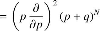
![$\displaystyle =\left(p\,\frac{\partial}{\partial p}\right)\left[p\,N\, (p+q)^{N-1}\right]$](img3441.png)
![$\displaystyle = p\left[N\,(p+q)^{N-1}+p\,N\,(N-1)\,(p+q)^{N-2}\right].$](img3442.png)

![$\displaystyle = p\left[N+p\,N\,(N-1)\right]= N\,p\left(1+p\,N-p\right)$](img3444.png)
