Next: Binomial Probability Distribution Up: Probability Theory Previous: Probability Theory
 . Suppose that a measurement of a given property of
this system can result in a number of distinct outcomes. If we wish to determine the
probability of obtaining a given outcome at an arbitrary time then we can take one of two approaches.
First, we can observe system at many distinct times; this approach is known as a
time average. Second, we can observe many systems that are identical to at an arbitrary time;
this approach is known as an ensemble average. An ensemble average is the most convenient theoretical approach,
and the one that we shall adopt in the following discussion,
whereas a time average is more directly related to real experiments.
. Suppose that a measurement of a given property of
this system can result in a number of distinct outcomes. If we wish to determine the
probability of obtaining a given outcome at an arbitrary time then we can take one of two approaches.
First, we can observe system at many distinct times; this approach is known as a
time average. Second, we can observe many systems that are identical to at an arbitrary time;
this approach is known as an ensemble average. An ensemble average is the most convenient theoretical approach,
and the one that we shall adopt in the following discussion,
whereas a time average is more directly related to real experiments.
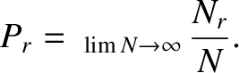
Suppose that there are  systems in our ensemble (i.e., collection of identical systems) and that
 of these systems exhibit the outcome
  . The probability of occurrence of outcome is
defined
. The probability of occurrence of outcome is
defined
 is a number that lies between 0 and 1. If
  then no systems in the ensemble
exhibit the outcome , even in the limit that the number of systems tends to infinity. This is another way
of saying that outcome is impossible. If
then no systems in the ensemble
exhibit the outcome , even in the limit that the number of systems tends to infinity. This is another way
of saying that outcome is impossible. If  then all systems in the ensemble exhibit the outcome ,
even in the limit that the number of systems tends to infinity. This is another way of saying that outcome
is certain to occur.
then all systems in the ensemble exhibit the outcome ,
even in the limit that the number of systems tends to infinity. This is another way of saying that outcome
is certain to occur.
Suppose that a measurement of a given property of some physical system can lead to any one of
 mutually exclusive outcomes. Let the total number of systems in the ensemble be , and
let the number of systems that exhibit the outcome be . It follows that
mutually exclusive outcomes. Let the total number of systems in the ensemble be , and
let the number of systems that exhibit the outcome be . It follows that
 |
(5.2) |
, and then take the limit that
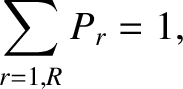
 , then we obtain the so-called normalization condition,
where use has been made of Equation (5.1). The normalization condition states that the sum of the probabilities of all
of the possible outcomes of a measurement of a given property of system is unity. This condition is equivalent to the self-evident proposition that a measurement of the property is bound to result in one of the possible outcomes of this measurement.
, then we obtain the so-called normalization condition,
where use has been made of Equation (5.1). The normalization condition states that the sum of the probabilities of all
of the possible outcomes of a measurement of a given property of system is unity. This condition is equivalent to the self-evident proposition that a measurement of the property is bound to result in one of the possible outcomes of this measurement.
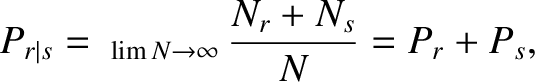
Let us determine the probability of occurrence of outcome or outcome  when an observation is made of our
system. Here, and are distinct outcomes. There are
when an observation is made of our
system. Here, and are distinct outcomes. There are  systems in our ensemble that
exhibit either the outcome or the outcome , so
systems in our ensemble that
exhibit either the outcome or the outcome , so
or the outcome is the sum of the probabilities of occurrence of these two outcomes.
For example, the probability
of throwing a  on a six-sided die is
  . Likewise, the probability of throwing a 2 is . Hence, the
probability of throwing a or a
. Likewise, the probability of throwing a 2 is . Hence, the
probability of throwing a or a  is
is
 . The previous result can easily be extended to deal
with more that two alternative outcomes.
. The previous result can easily be extended to deal
with more that two alternative outcomes.
Suppose that our system can exhibit two different types of outcome. Type-1 outcomes are labeled
 .
Type-2 outcomes are labeled
.
Type-2 outcomes are labeled
 . Let there be systems in our ensemble, and let of them
exhibit the type-1 outcome , and let
. Let there be systems in our ensemble, and let of them
exhibit the type-1 outcome , and let  of them exhibit the type-2 outcome . The probability of outcome is
 |
(5.5) |
 |
(5.6) |
is taken as read; see Equation (5.1).] By analogy, the number of systems that
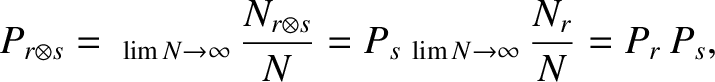
exhibit the type-1 outcome and the type-2 outcome is
 |
(5.7) |
and the type-2 outcome simultaneously is
where use has been made of Equation (5.1). However, the previous result is only valid provided outcomes
and are statistically independent of one another. In other words, obtaining the outcome must
not affect the probability of obtaining the outcome . As an example of the previous result, consider a
system consisting of two six-sided dies. The probability of throwing a 1 on either die is . Hence, the probability
of simultaneously throwing a 1 on both dies is
 . The previous result can easily be extended to
deal with more than two types of outcome.
. The previous result can easily be extended to
deal with more than two types of outcome.