Alternating current (AC) circuits are made up of voltage sources and three
different types of passive elements. These are resistors, inductors (i.e., small solenoids),
and capacitors. Resistors satisfy Ohm's law,
 |
(2.411) |
where  is the resistance,
  the current flowing through the resistor, and
 the voltage drop across the resistor (in the direction in which the current
flows). (See Section 2.1.11.) Inductors satisfy
the voltage drop across the resistor (in the direction in which the current
flows). (See Section 2.1.11.) Inductors satisfy
 |
(2.412) |
where  is the inductance. [See Equation (2.325).] Finally, capacitors obey
 |
(2.413) |
where  is the capacitance,
  is the charge stored on the plate with the most
positive potential, and
is the charge stored on the plate with the most
positive potential, and  for
for  . (See Section 2.1.13.) Note that any
passive component of a real electrical
circuit can always be represented as a combination of ideal resistors, inductors, and
capacitors.
. (See Section 2.1.13.) Note that any
passive component of a real electrical
circuit can always be represented as a combination of ideal resistors, inductors, and
capacitors.
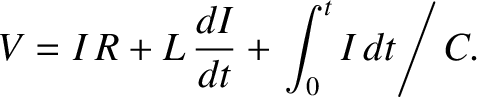
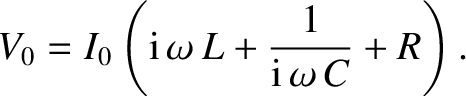
Let us consider the classic LCR circuit, which consists of an inductor, , a
capacitor, , and a resistor, , all connected in series with an voltage source,
. See Figure 2.35. The circuit equation is obtained by setting the input voltage equal to
the sum of the voltage drops across the three passive elements in the circuit.
Thus,
 |
(2.414) |
This is an integro-differential equation which, in general, is quite difficult to
solve. Suppose, however, that both the voltage and the current
oscillate at some fixed angular frequency,  , so that
where
, so that
where
 , and the physical solution is understood to be the real part of
the previous expressions. The assumed behavior of the voltage and current is
clearly relevant to electrical
circuits powered by mains electricity (which oscillates at 60 hertz in the U.S. and Canada).
, and the physical solution is understood to be the real part of
the previous expressions. The assumed behavior of the voltage and current is
clearly relevant to electrical
circuits powered by mains electricity (which oscillates at 60 hertz in the U.S. and Canada).
Figure 2.35:
An LCR circuit.
|
|
Equations (2.414)–(2.416) yield
 |
(2.417) |
giving
 |
(2.418) |
It is helpful to define the impedance of the circuit:
 |
(2.419) |
Impedance is a generalization of the concept of resistance. In general, the impedance
of an AC circuit is a complex quantity.
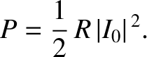
The average power output of the voltage source is
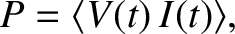 |
(2.420) |
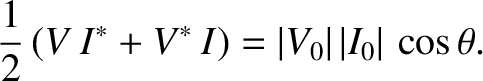
where the average is taken over one period of the oscillation. Let us, first of all,
calculate the power using real (rather than complex) voltages and currents.
We can write
where  is the phase-lag of the current with respect to the voltage.
It follows that
giving
is the phase-lag of the current with respect to the voltage.
It follows that
giving
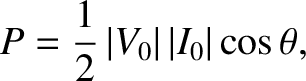 |
(2.424) |
because
 and
and
 . Here,
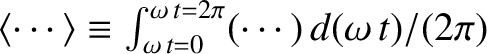 .
In complex representation, the voltage and the current are written
Now,
.
In complex representation, the voltage and the current are written
Now,
 |
(2.427) |
It follows from Equation (2.424) that
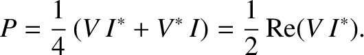 |
(2.428) |
Making use of Equation (2.419), we find that
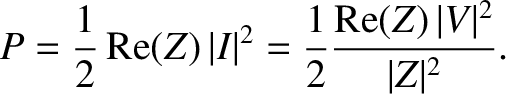 |
(2.429) |
Note that power dissipation is associated with the real part of the impedance.
For the specific case of an LCR circuit,
 |
(2.430) |
[See Equation (2.419).]
We conclude that only the resistor dissipates energy in this circuit. The inductor and
the capacitor both store energy, but they eventually return it to the circuit
without dissipation.
According to Equation (2.419), the amplitude of the current that flows in an LCR circuit,
for a given amplitude of the input voltage, is
given by
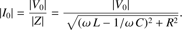 |
(2.431) |
As can be seen from Figure 2.36, the response of the circuit is
resonant, peaking at
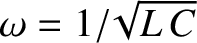 , and reaching
 of the peak value at
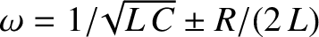 (assuming that
 ). For this reason, LCR circuits are used in analog radio tuners to filter out
signals whose frequencies fall outside a given band.
). For this reason, LCR circuits are used in analog radio tuners to filter out
signals whose frequencies fall outside a given band.
Figure: 2.36
The characteristics of an LCR circuit. The left-hand and right-hand panes show the amplitude and phase-lag of the current versus frequency, respectively. Here,
 and
and
 . The solid, short-dashed, long-dashed,
and dot-dashed curves correspond to
. The solid, short-dashed, long-dashed,
and dot-dashed curves correspond to  , 1/2, 1/4, and 1/8, respectively.
|
|
The phase-lag of the current with respect to the voltage is given by
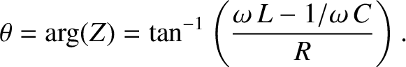 |
(2.432) |
[See Equation (2.419).]
As can be seen from Figure 2.36, the phase-lag varies from  for frequencies significantly below the resonant
frequency, to zero at the resonant frequency (
), to
for frequencies significantly below the resonant
frequency, to zero at the resonant frequency (
), to
 for frequencies significantly above the resonant frequency.
It is clear that, in conventional AC circuits, the circuit equation reduces to a
simple algebraic equation, and that the behavior of the circuit is summed up
by the complex impedance,  . The real part of tells us the power dissipated in
the circuit, the magnitude of gives the ratio of the peak current to the
peak voltage, and the argument of gives the phase-lag of the current
with respect to the voltage.
. The real part of tells us the power dissipated in
the circuit, the magnitude of gives the ratio of the peak current to the
peak voltage, and the argument of gives the phase-lag of the current
with respect to the voltage.


![$\displaystyle = \vert V_0\vert\, \vert I_0\vert \int_{\omega \,t =0}^{\omega\, ...
... \cos\theta + \sin(\omega \,t) \,\sin \theta\right]
\frac{d(\omega\, t)}{2\pi},$](img1956.png)
![$\displaystyle = \vert I_0\vert\, \exp[{\rm i}\,(\omega \,t - \theta)].$](img1962.png)
![\includegraphics[height=2.75in]{Chapter03/fig7_6.eps}](img1972.png)
![\includegraphics[height=2.5in]{Chapter03/fig7_5.eps}](img1947.png)