


Next: Infinite Spherical Potential Well
Up: Central Potentials
Previous: Introduction
Derivation of Radial Equation
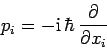
Now, we have seen that the Cartesian components of the momentum,  ,
can be represented as (see Sect. 7.2)
,
can be represented as (see Sect. 7.2)
 |
(624) |
for  , where
  ,
,  ,
,  , and
, and
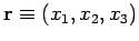 . Likewise, it is easily demonstrated,
from the above expressions, and the basic definitions of the spherical polar coordinates
[see Eqs. (545)-(550)], that the radial component
of the momentum can be represented as
. Likewise, it is easily demonstrated,
from the above expressions, and the basic definitions of the spherical polar coordinates
[see Eqs. (545)-(550)], that the radial component
of the momentum can be represented as
 |
(625) |
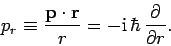
Recall that the angular momentum vector,  , is defined [see Eq. (526)]
 |
(626) |
This expression can also be written in the following form:
 |
(627) |
Here, the
 (where
  all run from 1 to 3) are
elements of the so-called totally anti-symmetric tensor. The values of
the various
elements of this tensor are determined via a simple rule:
all run from 1 to 3) are
elements of the so-called totally anti-symmetric tensor. The values of
the various
elements of this tensor are determined via a simple rule:
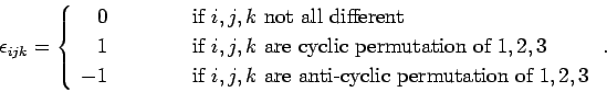 |
(628) |
Thus,
 ,
,
 , and
, and
 , etc.
Equation (627) also makes use of the Einstein summation
convention, according to which repeated indices are summed (from
1 to 3). For instance,
, etc.
Equation (627) also makes use of the Einstein summation
convention, according to which repeated indices are summed (from
1 to 3). For instance,
 .
Making use of this convention, as well as Eq. (628), it
is easily seen that Eqs. (626) and (627) are indeed equivalent.
.
Making use of this convention, as well as Eq. (628), it
is easily seen that Eqs. (626) and (627) are indeed equivalent.
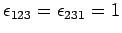
Let us calculate the value of  using Eq. (627). According
to our new notation, is the same as
using Eq. (627). According
to our new notation, is the same as  . Thus, we
obtain
. Thus, we
obtain
 |
(629) |
Note that we are able to shift the position of
 because its
elements are just numbers, and, therefore, commute with all of
the
because its
elements are just numbers, and, therefore, commute with all of
the  and the
  . Now, it is easily demonstrated that
 |
(630) |
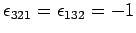
Here  is the usual Kronecker delta, whose elements
are determined according to the rule
is the usual Kronecker delta, whose elements
are determined according to the rule
![\begin{displaymath}
\delta_{ij} = \left\{
\begin{array}{rcl}
1 &\mbox{\hspace{1c...
...box{if $i$ and $j$ different}\ [0.5ex]
\end{array}\right. .
\end{displaymath}](img1513.png) |
(631) |
It follows from Eqs. (629) and (630) that
 |
(632) |
Here, we have made use of the fairly self-evident result that
 . We have also been careful to preserve the order of
the various terms on the right-hand side of the above expression, since the and the do not necessarily
commute with one another.
. We have also been careful to preserve the order of
the various terms on the right-hand side of the above expression, since the and the do not necessarily
commute with one another.
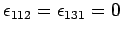
We now need to rearrange the order of the terms on the right-hand
side of Eq. (632). We can achieve this by making use of
the fundamental commutation relation for the and the [see Eq. (483)]:
![\begin{displaymath}[x_i,p_j]= {\rm i} \hbar \delta_{ij}.
\end{displaymath}](img1516.png) |
(633) |
Thus,
Here, we have made use of the fact that
 , since
the commute with one another [see Eq. (482)].
Next,
, since
the commute with one another [see Eq. (482)].
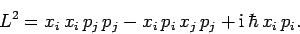
Next,
![\begin{displaymath}
L^2 = x_i x_i p_j p_j - x_i p_i\left(x_j p_j - [x_j,p_j]\right) - 2 {\rm i} \hbar x_i p_i.
\end{displaymath}](img1522.png) |
(635) |
Now, according to (633),
![\begin{displaymath}[x_j,p_j]\equiv [x_1,p_1]+[x_2,p_2]+[x_3,p_3] = 3 {\rm i} \hbar.
\end{displaymath}](img1523.png) |
(636) |
Hence, we obtain
 |
(637) |
When expressed in more conventional vector notation, the above expression
becomes
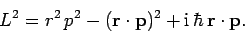 |
(638) |
Note that if we had attempted to derive the above expression
directly from Eq. (626), using standard vector identities, then we would have missed
the final term on the right-hand side. This term originates from the lack
of commutation between the and operators in quantum mechanics. Of course, standard
vector analysis assumes that all terms commute with one another.
Equation (638) can be rearranged to give
![\begin{displaymath}
p^2 = r^{-2}\left[({\bf r}\cdot{\bf p})^2- {\rm i} \hbar {\bf r}\cdot{\bf p}+L^2\right].
\end{displaymath}](img1526.png) |
(639) |
Now,
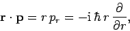 |
(640) |
where use has been made of Eq. (625). Hence, we obtain
![\begin{displaymath}
p^2 = -\hbar^2\left[\frac{1}{r}\frac{\partial}{\partial r}\l...
...}\frac{\partial}{\partial r}- \frac{L^2}{\hbar^2 r^2}\right].
\end{displaymath}](img1528.png) |
(641) |
Finally, the above equation can be combined with Eq. (623)
to give the following expression for the Hamiltonian:
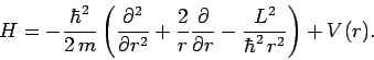 |
(642) |
Let us now consider whether the above Hamiltonian commutes with
the angular momentum operators  and . Recall, from
Sect. 8.3, that and are represented as differential
operators which depend solely on the angular spherical polar
coordinates,
and . Recall, from
Sect. 8.3, that and are represented as differential
operators which depend solely on the angular spherical polar
coordinates,  and
and  , and do not contain the radial
polar coordinate,
, and do not contain the radial
polar coordinate,  . Thus, any function of , or any differential
operator involving (but not and ), will automatically
commute with and . Moreover, commutes
both with itself, and with (see Sect. 8.2). It
is, therefore, clear that the above Hamiltonian commutes with
both and .
. Thus, any function of , or any differential
operator involving (but not and ), will automatically
commute with and . Moreover, commutes
both with itself, and with (see Sect. 8.2). It
is, therefore, clear that the above Hamiltonian commutes with
both and .
Now, according to Sect. 4.10, if two operators commute with
one another then they possess simultaneous eigenstates. We thus conclude
that for a particle moving in a central potential the eigenstates of the
Hamiltonian are simultaneous eigenstates of and .
Now, we have already found the simultaneous eigenstates of
and --they are the spherical harmonics,
 ,
discussed in Sect. 8.7. It follows that the spherical
harmonics are also eigenstates of the Hamiltonian. This observation leads
us to try the following separable form for the stationary
wavefunction:
,
discussed in Sect. 8.7. It follows that the spherical
harmonics are also eigenstates of the Hamiltonian. This observation leads
us to try the following separable form for the stationary
wavefunction:
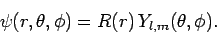 |
(643) |
It immediately follows, from (556) and (557), and the
fact that and both obviously commute with  , that
Recall that the quantum numbers  and
and  are restricted to take certain
integer values, as explained in Sect. 8.6.
are restricted to take certain
integer values, as explained in Sect. 8.6.
Finally, making use of Eqs. (622), (642), and (645),
we obtain the following differential equation which determines the radial variation of the stationary wavefunction:
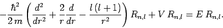 |
(646) |
Here, we have labeled the function by two quantum numbers,
 and . The second quantum number, , is, of course, related to the eigenvalue of . [Note that
the azimuthal quantum number, , does not appear in the above equation,
and, therefore, does not influence either the function or the energy,
and . The second quantum number, , is, of course, related to the eigenvalue of . [Note that
the azimuthal quantum number, , does not appear in the above equation,
and, therefore, does not influence either the function or the energy,  .] As we shall see, the first quantum number, , is determined by the constraint that the radial wavefunction be square-integrable.
Next: Infinite Spherical Potential Well
Up: Central Potentials
Previous: Introduction
Richard Fitzpatrick
2010-07-20