


Next: Particle in a Box
Up: Three-Dimensional Quantum Mechanics
Previous: Introduction
Fundamental Concepts
We have seen that in one dimension the instantaneous state
of a single non-relativistic particle is fully specified by a complex wavefunction,
 . The probability
of finding the particle at time
. The probability
of finding the particle at time  between
  and
and  is
is
 , where
 |
(467) |
Moreover, the wavefunction is
normalized such that
 |
(468) |
at all times.
In three dimensions, the instantaneous state of a single particle is also
fully specified by a complex wavefunction,  .
By analogy with the one-dimensional case, the probability of finding
the particle at time between and , between
.
By analogy with the one-dimensional case, the probability of finding
the particle at time between and , between  and
and  , and between
 and
and  , is
, is
 , where
 |
(469) |
As usual, this interpretation of the wavefunction only makes sense if the
wavefunction is normalized such that
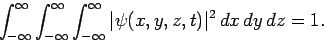 |
(470) |
This normalization constraint ensures that the probability of finding the particle anywhere is space is always unity.
In one dimension, we can write the probability conservation equation (see
Sect. 4.5)
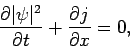 |
(471) |
where
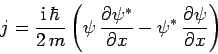 |
(472) |
is the flux of probability along the -axis. Integrating
Eq. (471) over all space, and making use of the fact that
 as
as
 if
if  is to be square-integrable, we obtain
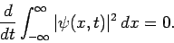 |
(473) |
In other words, if the wavefunction is initially normalized then it stays
normalized as time progresses. This is a necessary criterion for the viability of our basic
interpretation of  as a probability density.
In three dimensions, by analogy with the one dimensional case, the probability conservation equation becomes
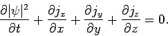 |
(474) |
Here,
 |
(475) |
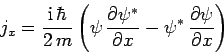
is the flux of probability along the -axis, and
 |
(476) |
the flux of probability along the -axis, etc.
Integrating
Eq. (474) over all space, and making use of the fact that
as
 if is to be square-integrable, we obtain
 |
(477) |
Thus, the normalization of the wavefunction is again preserved as time
progresses, as must be the case if is to be interpreted as a
probability density.
In one dimension, position is represented by the algebraic operator ,
whereas momentum is represented by the differential operator
 (see Sect. 4.6). By analogy, in
three dimensions, the Cartesian coordinates , , and
are represented by the algebraic operators , , and ,
respectively, whereas the three Cartesian components of momentum,
(see Sect. 4.6). By analogy, in
three dimensions, the Cartesian coordinates , , and
are represented by the algebraic operators , , and ,
respectively, whereas the three Cartesian components of momentum,
 ,
,  , and
, and  , have the following representations:
Let  ,
,  ,
,  , and
, and  , etc.
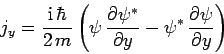
Since the
, etc.
Since the  are independent variables (i.e.,
 ), we conclude that the
various position and momentum operators satisfy the following commutation
relations:
), we conclude that the
various position and momentum operators satisfy the following commutation
relations:
Now, we know, from Sect. 4.10, that two dynamical variables
can only be (exactly) measured simultaneously if the operators which represent
them in quantum mechanics commute with one another. Thus,
it is clear, from the above commutation relations, that the only restriction
on measurement in a system consisting of a single particle moving in
three dimensions is that it is impossible to
simultaneously measure a given position coordinate and the corresponding
component of momentum. Note, however, that it is perfectly possible to
simultaneously measure two different positions coordinates, or two
different components of the momentum. The commutation
relations (481)-(483) again illustrate the
point that quantum mechanical operators corresponding to different degrees of freedom of a
dynamical system (in this case, motion in different directions) tend to commute
with one another (see Sect. 6.2).
In one dimension, the time evolution of the wavefunction is given
by [see Eq. (199)]
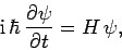 |
(484) |
where
 is the Hamiltonian. The same equation
governs the time evolution of the wavefunction in three dimensions.
is the Hamiltonian. The same equation
governs the time evolution of the wavefunction in three dimensions.
Now, in one dimension, the Hamiltonian of a non-relativistic particle
of mass  takes the form
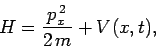 |
(485) |
where  is the potential energy. In three dimensions, this expression
generalizes to
is the potential energy. In three dimensions, this expression
generalizes to
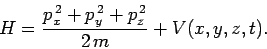 |
(486) |
Hence, making use of Eqs. (478)-(480) and (484), the three-dimensional version of the time-dependent Schröndiger equation
becomes [see Eq. (137)]
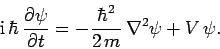 |
(487) |
Here, the differential operator
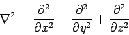 |
(488) |
is known as the Laplacian. Incidentally, the probability conservation equation
(474) is easily derivable from Eq. (487).
An eigenstate of the Hamiltonian corresponding
to the eigenvalue  satisfies
 |
(489) |
It follows from Eq. (484) that (see Sect. 4.12)
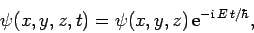 |
(490) |
where the stationary wavefunction  satisfies the
three-dimensional version of the time-independent Schröndiger equation
[see Eq. (295)]:
satisfies the
three-dimensional version of the time-independent Schröndiger equation
[see Eq. (295)]:
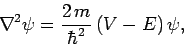 |
(491) |
where  is assumed not to depend explicitly on .
Next: Particle in a Box
Up: Three-Dimensional Quantum Mechanics
Previous: Introduction
Richard Fitzpatrick
2010-07-20


