General Paramagnetism

In Section 7.3, we considered the special case of paramagnetism in which all the atoms that make up the substance under investigation possess spin 1/2. Let us now discuss the general case.

Consider a system consisting of $N$ non-interacting atoms in a substance held at absolute temperature $T$ , and placed in an external magnetic field, ${\bf B} = B_z {\bf e}_z$ , that points in the $z$ -direction. The magnetic energy of a given atom is written

$$\epsilon = - \mbox{\boldmath$\mu$} \cdot{\bf B},$$ (7.91)

where $\mu$ is the atom's magnetic moment. Now, the magnetic moment of an atom is proportional to its total electronic angular momentum, $\hbar {\bf J}$ . In fact,

$$\mbox{\boldmath$\mu$} =g \mu_B {\bf J},$$ (7.92)

where

$$\mu_B = \frac{e \hbar}{2 m_e}$$ (7.93)

is a standard unit of magnetic moment known as the Bohr magneton. Here, $e$ is the magnitude of the electron charge, and $m_e$ the electron mass. Moreover, $g$ is a dimensionless number of order unity that is called the g-factor of the atom.

Combining Equations (7.91) and (7.92), we obtain

$$\epsilon = -g \mu_B {\bf J}\cdot{\bf B} = -g \mu_B B_z J_z.$$ (7.94)

Now, according to standard quantum mechanics,

$$J_z=m,$$ (7.95)

where $m$ is an integer that can take on all values between $-J$ and $+J$ . Here, $\vert{\bf J}\vert=J (J+1)$ , where $J$ is a positive number that can either take integer or half-integer values. Thus, there are $2 J+1$ allowed values of $m$ , corresponding to different possible projections of the angular momentum vector along the $z$ -direction. It follows from Equation (7.94) that the possible magnetic energies of an atom are

$$\epsilon_m = -g \mu_B B_z m.$$ (7.96)

For example, if $J=1/2$ (corresponding to a spin-1/2 system) then there are only two possible energies, corresponding to $m=\pm 1/2$ . This was the situation considered in Section 7.3. (To be more exact, a spin-1/2 system corresponds to $J=1/2$ and $g=2$ .)

The probability, $P_m$ , that an atom is in a state labeled $m$ is

$$P_m\propto \exp(-\beta \epsilon_m)=\exp( \beta g \mu_B B_z m),$$ (7.97)

where $\beta = 1/(k T)$ . According to Equation (7.92), the corresponding $z$ -component of the magnetic moment is

$$\mu_z=g \mu_B m.$$ (7.98)

Hence, the mean $z$ -component of the magnetic moment is

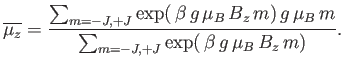$$\overline{\mu_z} =\frac{\sum_{m=-J,+J}\exp( \beta g \mu_B B_z m) g \mu_B m}{\sum_{m=-J,+J}\exp( \beta g \mu_B B_z m)}.$$ (7.99)

The numerator in the previous expression is conveniently expressed as a derivative with respect to the external parameter $B_z$ :

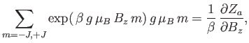$$\sum_{m=-J,+J}\exp( \beta g \mu_B B_z m) g \mu_B m=\frac{1}{\beta} \frac{\partial Z_a}{\partial B_z},$$ (7.100)

where

$$Z_a =\sum_{m=-J,+J} \exp( \beta g \mu_B B_z m)$$ (7.101)

is the partition function of a single atom. Thus, Equation (7.99) becomes

$$\overline{\mu_z} =\frac{1}{Z_a} \frac{1}{\beta} \frac{\partial Z_a}{\partial B_z}=\frac{1}{\beta} \frac{\partial \ln Z_a}{\partial B_z}.$$ (7.102)

In order to calculate $Z_a$ , it is convenient to define

$$\eta= \beta g \mu_B B_z = \frac{g \mu_B B_z}{k T},$$ (7.103)

which is a dimensionless parameter that measures the ratio of the magnetic energy, $g \mu_B B_z$ , that acts to align the atomic magnetic moments parallel to the external magnetic field, to the thermal energy, $k T$ , that acts to keep the magnetic moment randomly orientated. Thus, Equation (7.101) becomes

$$Z_a =\sum_{m=-J,+J}\exp(m \eta)= {\rm e}^{-\eta J}\sum_{k=0,2J}[\exp(\eta)]^{ k}.$$ (7.104)

The previous geometric series can be summed to give

$$Z_a = {\rm e}^{-\eta J}\left\{\frac{1-[\exp(\eta)]^{ 2J+1}}{1-\exp(\eta)}\right\}.$$ (7.105)

(See Exercise 1.) Multiplying the numerator and denominator by $\exp(-\eta/2)$ , we obtain

$$Z_a = \frac{\exp[-\eta (J+1/2)]+\exp[ \eta (J+1/2)]}{\exp(-\eta/2)-\exp( \eta/2)},$$ (7.106)

or

$$Z_a =\frac{\sinh[(J+1/2) \eta]}{\sinh(\eta/2)},$$ (7.107)

where the hyperbolic sine is defined

$$\sinh z \equiv \frac{\exp( y)-\exp(-y)}{2}.$$ (7.108)

Thus,

$$\ln Z_a =\ln \sinh[(J+1/2) \eta]-\ln\sinh(\eta/2).$$ (7.109)

According to Equations (7.102) and (7.103),

$$\overline{\mu_z} =\frac{1}{\beta} \frac{\partial \ln Z_a}{\parti... ...{\partial\eta}{\partial B_z} =g \mu_B \frac{\partial \ln Z_a}{\partial\eta}.$$ (7.110)

Hence,

$$\overline{\mu_z} = g \mu_B\left\{\frac{(J+1/2) \cosh[(J+1/2) \eta]}{\sinh[(J+1/2) \eta]}-\frac{(1/2) \cosh(\eta/2)}{\sinh(\eta/2)}\right\},$$ (7.111)

or

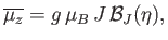$$\overline{\mu_z} = g \mu_B J {\cal B}_J(\eta),$$ (7.112)

where

$${\cal B}_J(\eta) =\frac{1}{J}\left\{\left(J+\frac{1}{2}\right)\co... ...c{1}{2}\right)\eta\right]-\frac{1}{2} \coth\left(\frac{\eta}{2}\right)\right\}$$ (7.113)

is known as the Brillouin function.

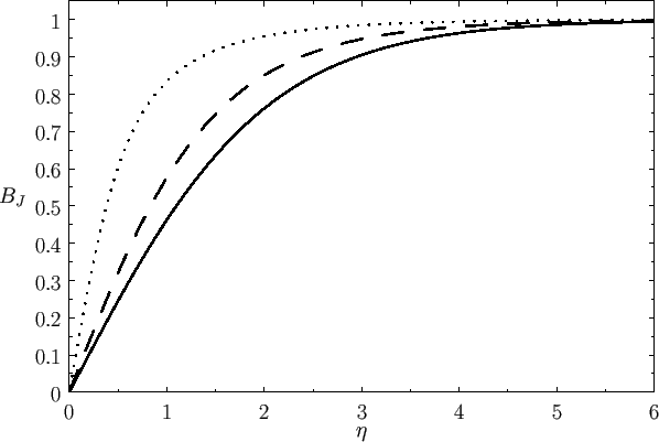
Figure: The solid, dashed, and dotted curves show the Brillouin function, ${\cal B}_J(\eta )$ , for $J=1/2$ , $J=1$ , and $J=7/2$ , respectively.

The hyperbolic cotangent is defined

$$\coth z \equiv \frac{\cosh z}{\sinh z}=\frac{\exp( z)+\exp(-z)}{\exp( z)-\exp(-z)}.$$ (7.114)

For $z\gg 1$ , we have

$$\coth z\simeq 1.$$ (7.115)

On the other hand, for $z\ll 1$ ,

$$\coth z = \frac{1}{z}+\frac{1}{3} z + {\cal O}\left(z^{ 3}\right).$$ (7.116)

Thus, it follows that

$${\cal B}_J(\eta)= \frac{1}{J}\left[\left(J+\frac{1}{2}\right)-\frac{1}{2}\right] = 1$$ (7.117)

when $\eta\gg 1$ . On the other hand, when $\eta\ll 1$ , we get

$${\cal B}_J(\eta) =\frac{1}{J}\left\{\left(J+\frac{1}{2}\right)\left[\frac{1}{(J+1/... ...right)\eta\right]-\frac{1}{2}\left(\frac{2}{\eta}+\frac{\eta}{6}\right)\right\}$$

$$=\frac{1}{J}\left[\frac{1}{3}\left(J+\frac{1}{2}\right)^{ 2}\eta... ...} \eta\right]=\frac{\eta}{3 J}\left(J^{ 2}+J+\frac{1}{4}-\frac{1}{4}\right),$$ (7.118)

which reduces to

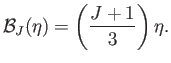$${\cal B}_J(\eta) = \left(\frac{J+1}{3}\right)\eta.$$ (7.119)

Figure 7.1 shows how ${\cal B}_J(\eta )$ depends on $\eta$ for various values of $J$ .

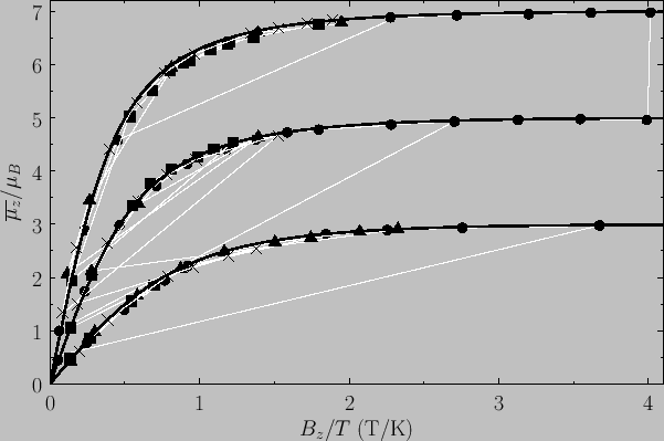
Figure: The magnetization versus $B_z/T$ curves for (lower curve) chromium potassium alum ($J=3/2$ , $g=2$ ), (middle curve) iron ammonium alum ($J=5/2$ , $g=2$ ), and (top curve) gadolinium sulphate ($J=7/2$ , $g=2$ ). The solid lines are the theoretical predictions, whereas the data points are experimental measurements. The circles, triangles, crosses, and squares correspond to $T=1.30$ K, $2.00$ K, $3.00$ K, and $4.21$ K, respectively. From W.E. Henry, Phys. Rev. 88, 561 (1952).

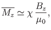
If there are $N_0$ atoms per unit volume then the mean magnetic moment per unit volume (or magnetization) becomes

$$\overline{M_z} = N_0 \overline{\mu_z} = N_0 g \mu_B J {\cal B}_J(\eta),$$ (7.120)

where use has been made of Equation (7.112). If $\eta\ll 1$ then Equation (7.119) implies that $\overline{M_z}\propto \eta\propto B_z/T$ . This relation can be written

$$\overline{M_z} \simeq \chi \frac{B_z}{\mu_0},$$ (7.121)

where the dimensionless constant of proportionality,

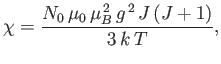$$\chi =\frac{N_0 \mu_0 \mu_B^{ 2} g^{ 2} J (J+1)}{3 k T},$$ (7.122)

is known as the magnetic susceptibility. Thus, $\chi\propto T^{ -1}$ --a result that is called Curie's law. (See Section 7.3.) If $\eta\gg 1$ then

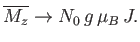$$\overline{M_z}\rightarrow N_0 g \mu_B J.$$ (7.123)

This corresponds to magnetic saturation--a situation in which each atom has the maximum component of the magnetic moment parallel to the magnetic field, $g \mu_B J$ , that it can possibly have.

Figure 7.2 compares the experimental and theoretical magnetization versus field-strength curves for three different paramagnetic substances containing atoms of total angular momentum $3/2$ , $5/2$ , and $7/2$ particles, showing excellent agreement between theory and experiment. Note that, in all cases, the magnetization is proportional to the magnetic field-strength at small field-strengths, but saturates at some constant value as the field-strength increases.

The previous analysis completely neglects any interaction between the spins of neighboring atoms or molecules. It turns out that this is a fairly good approximation for paramagnetic substances. However, for ferromagnetic substances, in which the spins of neighboring atoms interact very strongly, this approximation breaks down completely. (See Section 7.17.) Thus, the previous analysis does not apply to ferromagnetic substances.