


Next: Exercises
Up: Applications of Statistical Thermodynamics
Previous: Effusion
Ferromagnetism
Consider a solid substance consisting of  identical atoms arranged in a regular lattice. Each atom has
a net electronic angular momentum,
identical atoms arranged in a regular lattice. Each atom has
a net electronic angular momentum,
 , and an associated magnetic moment,
 . [Here, we use
  , rather than
 , to denote atomic angular momentum (divided by
  ) to avoid confusion with the exchange energy,
  , introduced in Equation (7.246).]
The atomic magnetic moment is related to the corresponding total angular momentum via
, introduced in Equation (7.246).]
The atomic magnetic moment is related to the corresponding total angular momentum via
  |
(7.244) |
where  is the Bohr magneton, and the
  -factor,
, is a dimensionless number of order unity. (See Section 7.9.)
In the presence of an externally-applied magnetic field,
-factor,
, is a dimensionless number of order unity. (See Section 7.9.)
In the presence of an externally-applied magnetic field,
 , directed parallel to the
  -axis, the Hamiltonian,
  ,
representing the interaction of the atoms with this field is written
,
representing the interaction of the atoms with this field is written
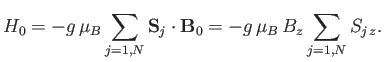 |
(7.245) |
Each atom is also assumed to interact with neighboring atoms. The interaction in question is not simply the
magnetic dipole-dipole interaction due to the magnetic field produced by one atom at the position of another.
Such an interaction is, in general, much too small to produce ferromagnetism. Instead, the predominant interaction is known as
the exchange interaction. This interaction is a quantum-mechanical consequence of the Pauli exclusion
principle. (See Section 8.2.) Because electrons cannot occupy the same state, two electrons on neighboring atoms
that have parallel spins (here, to simplify the discussion of the origin of the exchange interaction, we are temporarily assuming that the electrons all have zero orbital angular momenta, so that their
total angular momenta are solely a consequence of their spin angular momenta) cannot come too close to one another in space (else they would simultaneously occupy identical spin
and orbital states, which is forbidden). On the other hand, if the electrons have antiparallel spins then they are
in different spin states, so they are allowed to occupy the same orbital state. In other words, there is no exclusion-related
restriction on how close they can come together. Because different spatial separations of the electrons
give rise to different electrostatic interaction between them, the electrostatic interaction
between neighboring atoms (which is much stronger than any magnetic interaction) depends on the relative
orientations of their spins. This, then, is the origin of the exchange interaction, which for two atoms labelled  and
and  can be written in the form
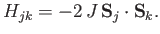 |
(7.246) |
Here, the so-called exchange energy,
, is a parameter (with the dimensions of energy) that depends on the atomic separation, and which measures the strength of the exchange interaction.
If  then the interaction energy is lower when spins on neighboring atoms are parallel, rather than antiparallel.
This state of affairs favors parallel spin alignment of neighboring atoms. In other words, it tends to produce ferromagnetism. Note
that, because the exchange interaction depends on the degree to which the electron orbitals of the two atoms can overlap, so
as to occupy approximately the same region of space, the exchange energy,
, falls off very rapidly with increasing atomic separation.
Hence, a given atom only interacts appreciably with its
then the interaction energy is lower when spins on neighboring atoms are parallel, rather than antiparallel.
This state of affairs favors parallel spin alignment of neighboring atoms. In other words, it tends to produce ferromagnetism. Note
that, because the exchange interaction depends on the degree to which the electron orbitals of the two atoms can overlap, so
as to occupy approximately the same region of space, the exchange energy,
, falls off very rapidly with increasing atomic separation.
Hence, a given atom only interacts appreciably with its  (say) nearest neighbors.
To simplify the interaction problem, we shall replace the previous expression by the simpler functional
form
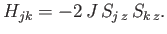 |
(7.247) |
This approximate expression, which is known as the Ising model, leaves the essential physical situation intact, while avoiding the complications introduced by
vector quantities. The Ising model is equivalent to assuming that all atomic magnetic moments are either directed parallel or anti-parallel to the
-axis.
The Hamiltonian,  , representing the interaction energy between atoms is written in the form
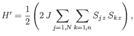 |
(7.248) |
where
is the exchange energy for neighboring atoms, and the index
refers to the nearest neighbor shell
surrounding the atom
. The factor  is introduced because the interaction between the same two atoms is counted twice in performing the sums.
The total Hamiltonian of the atoms is
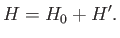 |
(7.249) |
The task in hand is to calculate the mean magnetic moment of the system parallel to the applied magnetic field,
 , as a function of its absolute temperature,
  , and the
applied field,
, and the
applied field,  . The presence of the interatomic interactions makes this task difficult, despite the extreme
simplicity of expression (7.248). Although the problem has been solved exactly for a linear one-dimensional array of atoms, and for two-dimensional
array of atoms when
. The presence of the interatomic interactions makes this task difficult, despite the extreme
simplicity of expression (7.248). Although the problem has been solved exactly for a linear one-dimensional array of atoms, and for two-dimensional
array of atoms when  , the three-dimensional problem is so complex that no exact solution has ever been found.
Thus, in order to make further progress, we must introduce an additional approximation.
, the three-dimensional problem is so complex that no exact solution has ever been found.
Thus, in order to make further progress, we must introduce an additional approximation.
Let us focus attention on a particular atom,
, which we shall refer to as the ``central atom.'' The interactions of this
atom are described by the Hamiltonian
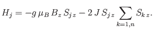 |
(7.250) |
The final term represents the interaction of the central atom with its nearest neighbors. As a simplifying approximation,
we shall replace the sum over these neighbors by its mean value. In other words, we shall write
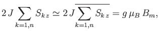 |
(7.251) |
where  is a parameter with the dimensions of magnetic field-strength, which is called the molecular field, and is
to be determined in such a way that it leads to a self-consistent solution of the statistical problem. In terms of this parameter,
expression (7.250) becomes
is a parameter with the dimensions of magnetic field-strength, which is called the molecular field, and is
to be determined in such a way that it leads to a self-consistent solution of the statistical problem. In terms of this parameter,
expression (7.250) becomes
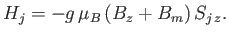 |
(7.252) |
Thus, the influence of neighboring atoms has been replaced by an effective magnetic field,
. The problem
presented by expression (7.252) reduces to the elementary one of a single atom, of normalized angular momentum,  , and
-factor,
, placed in an external
-directed magnetic
field,
, and
-factor,
, placed in an external
-directed magnetic
field,  . Recall, however, that we already solved this problem in Section 7.9.
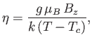
According to the analysis of Section 7.9,
 |
(7.253) |
where
 |
(7.254) |
and
 . Here,
 is the Brillouin function, for normalized atomic angular momentum
, that was introduced in Equation (7.113).
is the Brillouin function, for normalized atomic angular momentum
, that was introduced in Equation (7.113).
Expression (7.253) involves the unknown parameter
. To determine the value of this parameter in a
self-consistent manner, we note that there is nothing that distinguishes the central
th atom from any
of its neighboring atoms. Hence, any one of these atoms might equally well have been considered the central
atom. Thus, the corresponding mean value
 is also given by Equation (7.253).
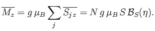
It follows from Equations (7.251) and (7.253) that
is also given by Equation (7.253).
It follows from Equations (7.251) and (7.253) that
 |
(7.255) |
The previous two equations can be combined to give
 |
(7.256) |
which determines  (and, hence,
). Once
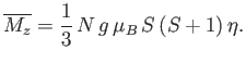
has been found, the mean magnetic moment
of the system follows from Equation (7.253):
(and, hence,
). Once
has been found, the mean magnetic moment
of the system follows from Equation (7.253):
 |
(7.257) |
Figure:
Graphical solution of Equation (7.256) that determines the molecular field,
, corresponding
to the intersection of the curves at
 . The dash-dotted straight-line corresponds to the case where the
external magnetic field,
, is zero.
. The dash-dotted straight-line corresponds to the case where the
external magnetic field,
, is zero.
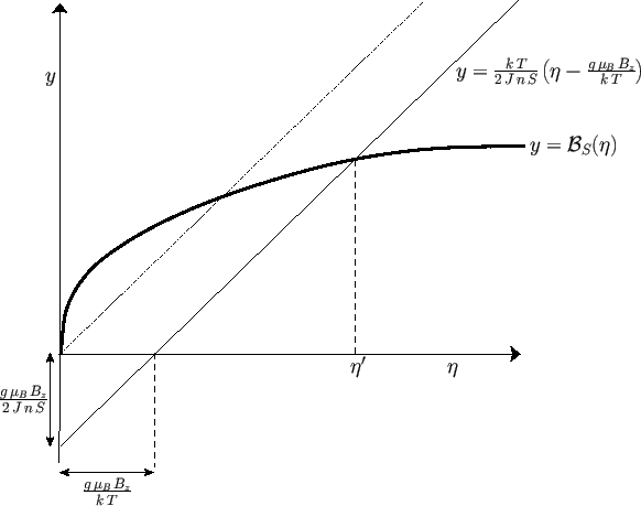 |
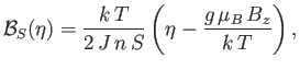
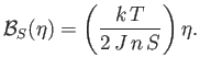
The solution of Equation (7.256) can be found by drawing, on the same graph, both the
Brillouin function
 and the straight-line
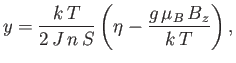 |
(7.258) |
and then finding the point of intersection of the two curves. See Figure 7.9.
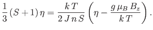
Consider the case where the external field,
, is zero. Equation (7.256) simplifies to
give
 |
(7.259) |
Given that
 , it follows that
  is a solution of the previous equation. This solution
is characterized by zero magnetization: that is,
is a solution of the previous equation. This solution
is characterized by zero magnetization: that is,
 . However, there is also
the possibility of another solution with
. However, there is also
the possibility of another solution with
 , and, hence,
 . (See Figure 7.9.)
The presence of such spontaneous magnetization in the absence of an external magnetic field is, of course, the distinguishing
feature of ferromagnetic materials. In order to have a solution with
, it is necessary that
the curves shown in Figure 7.9 intersect at a point
when both curves pass through the origin. The
condition for the existence of an intersection with
is that the slope of the curve
. (See Figure 7.9.)
The presence of such spontaneous magnetization in the absence of an external magnetic field is, of course, the distinguishing
feature of ferromagnetic materials. In order to have a solution with
, it is necessary that
the curves shown in Figure 7.9 intersect at a point
when both curves pass through the origin. The
condition for the existence of an intersection with
is that the slope of the curve
 at
should exceed that of the straight-line
at
should exceed that of the straight-line
 . In other words,
 |
(7.260) |
However, when  , the Brillouin function takes the simple form specified in Equation (7.119):
 |
(7.261) |
Hence, Equation (7.260) becomes
 |
(7.262) |
or
 |
(7.263) |
where
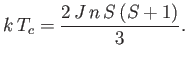 |
(7.264) |
Thus, we deduce that spontaneous magnetization of a ferromagnetic material is only possible
below a certain critical temperature,  , known as the Curie temperature. The
magnetized state, in which all atomic magnetic moments can exploit their mutual exchange energy by being
preferentially aligned parallel to one another, has a lower magnetic energy than the unmagnetized state
in which
. Thus, at temperatures below the
Curie temperature, the magnetized state is stable, whereas the unmagnetized state is unstable.
, known as the Curie temperature. The
magnetized state, in which all atomic magnetic moments can exploit their mutual exchange energy by being
preferentially aligned parallel to one another, has a lower magnetic energy than the unmagnetized state
in which
. Thus, at temperatures below the
Curie temperature, the magnetized state is stable, whereas the unmagnetized state is unstable.
As the temperature,
, is decreased below the Curie temperature,
, the slope of the
dash-dotted straight-line in Figure 7.9 decreases so that it intersects the curve
at increasingly large values of
. As
 , the intersection occurs at
 .
Because,
.
Because,
 [see Equation (7.117)], it follows from Equation (7.257) that
 as
. This corresponds to a state in which
all atomic magnetic moments are aligned completely parallel to one another. For temperatures,
, less than the
Curie temperature,
, we can use Equations (7.257) and (7.259) to compute
as
. This corresponds to a state in which
all atomic magnetic moments are aligned completely parallel to one another. For temperatures,
, less than the
Curie temperature,
, we can use Equations (7.257) and (7.259) to compute
 in the absence of an
external magnetic field.
We then obtain a magnetization curve of the general form shown in Figure 7.10.
in the absence of an
external magnetic field.
We then obtain a magnetization curve of the general form shown in Figure 7.10.
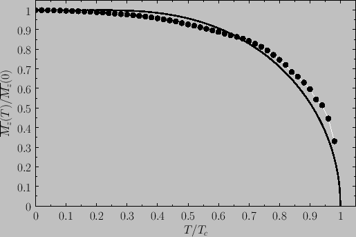
Figure:
Spontaneous magnetization of a ferromagnet as a function of the temperature in the presence of zero
external magnetic field. The solid curve is the prediction of molecular field theory for  and
and  . The
points are experimental data for nickel [from R. Kaul, and E.D. Thompson, J. appl. Phys. 40, 1383 (1969)].
. The
points are experimental data for nickel [from R. Kaul, and E.D. Thompson, J. appl. Phys. 40, 1383 (1969)].
 |
Let us, finally, investigate the magnetic susceptibility of a ferromagnetic substance, in the presence of a small external magnetic field, at temperatures
above the Curie temperature. In this case, the crossing point of the two curves in Figure 7.9 lies at small
. Hence,
we can use the approximation (7.261) to write Equation (7.256) in the form
 |
(7.265) |
Solving the previous equation for
gives
 |
(7.266) |
where use has been made of Equation (7.264). Now, making use of the approximation (7.261), Equation (7.257) reduces to
 |
(7.267) |
The previous two equations can be combined to give
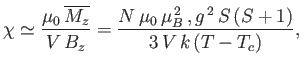 |
(7.268) |
where  is the dimensionless magnetic susceptibility of the substance, and
  is its volume.
This result is known as the Curie-Weiss law. It
differs from Curie's law,
is its volume.
This result is known as the Curie-Weiss law. It
differs from Curie's law,
 (see Section 7.3), because of the presence of the
parameter
in the denominator. According to the Curie-Weiss law,
becomes infinite when
(see Section 7.3), because of the presence of the
parameter
in the denominator. According to the Curie-Weiss law,
becomes infinite when
 : that is,
at the Curie temperature, when the substance becomes ferromagnetic.
: that is,
at the Curie temperature, when the substance becomes ferromagnetic.
Figure:
Plot of  (where
  is the mass density) versus temperature for gadolinium above its Curie temperature.
The curve is (apart from some slight departures at high temperatures) a straight-line, in accordance with the
Curie-Weiss law. The intercept of the line with the temperature axis gives
is the mass density) versus temperature for gadolinium above its Curie temperature.
The curve is (apart from some slight departures at high temperatures) a straight-line, in accordance with the
Curie-Weiss law. The intercept of the line with the temperature axis gives  K. The metal
becomes ferromagnetic below
K. The metal
becomes ferromagnetic below  K. Data from S. Arajs, and R.V. Colvin, J. appl. Phys. 32, 336S (1961).
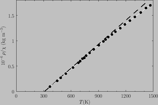 |
Experimentally, the Curie-Weiss law is well obeyed at temperatures significantly above the Curie temperature. See Figure 7.11.
It is, however, not true that the temperature,
, that occurs in this law is exactly the same as the Curie temperature
at which the substance becomes ferromagnetic.
The so-called Weiss molecular-field model (which was first put forward by Pierre Weiss in 1907) that we have just described is
remarkably successful at explaining the major features of ferromagnetism. Nevertheless, there are some serious discrepancies
between the predictions of this simple model and experimental data. In particular, the magnetic contribution to the
specific heat is observed to have a very sharp discontinuity at the Curie temperature (in the absence of an external field),
whereas the molecular field model predicts a much less abrupt change. Needless to say, more refined models have been
devised that considerably improve the agreement with experimental data.
Next: Exercises
Up: Applications of Statistical Thermodynamics
Previous: Effusion
Richard Fitzpatrick
2016-01-25