Composite Linear/Nonlinear Model

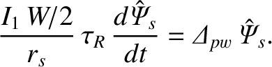
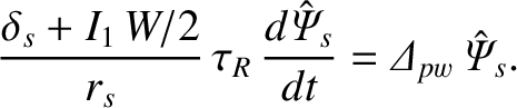
According to Equation (6.25), the time evolution of the reconnected magnetic flux (in a frame of reference that co-rotates with the magnetic island chain) in the linear regime is governed by

$$\frac{d\ln\hat{\mit\Psi}_s}{dt}\,\tau_R\,\frac{\delta_s}{r_s} = {\mit\Delta}_{pw},$$ (9.6)

where $\delta _s$ is the linear layer width. The previous equation can be rearranged to give

$$\frac{\delta_s}{r_s}\,\tau_R\,\frac{d\hat{\mit\Psi}_s}{dt} = {\mit\Delta}_{pw}\,\hat{\mit\Psi}_s.$$ (9.7)

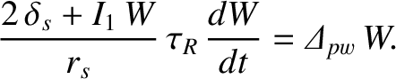
Now, given that $W\propto \hat{\mit\Psi}_s^{1/2}$ [see Equation (8.1)], the Rutherford island width evolution equation, (9.5), can be rewritten in the form

$$\frac{I_1\,W/2}{r_s}\,\tau_R\,\frac{d\hat{\mit\Psi}_s}{dt} = {\mit\Delta}_{pw}\,\hat{\mit\Psi}_s.$$ (9.8)

It can be seen, via a comparison between the previous two equations, that a nonlinear magnetic island chain evolves in time in an analogous fashion to a linear layer whose width is $I_1\,W/2$. In other words, the essential nonlinearity in the nonlinear regime comes about because the effective layer width is amplitude dependent.

Now, Equation (9.7) is valid when $\delta_s\gg W$ (i.e., when the linear layer width is much greater than the island width), whereas Equation (9.8) is valid in the opposite limit. This observation allows us to formulate a composite time evolution equation that encompasses both the linear and the nonlinear regimes [3,4,8,10]:

$$\frac{\delta_s + I_1\,W/2}{r_s}\,\tau_R \,\frac{d\hat{\mit\Psi}_s}{dt} = {\mit\Delta}_{pw}\,\hat{\mit\Psi}_s.$$ (9.9)

The previous equation can also be written

$$\frac{2\,\delta_s+I_1\,W}{r_s}\,\tau_R\,\frac{dW}{dt} = {\mit\Delta}_{pw}\,W.$$ (9.10)

Figure 9.1: Time evolution of the magnetic island width predicted by the composite linear/nonlinear model.

Let

$$\hat{W} = \frac{I_1\,W}{2\,\delta_s},$$ (9.11)

$$\hat{t} = \left(\frac{r_s\,{\mit\Delta}_{pw}}{2\,\delta_s\,\tau_R}\right)t.$$ (9.12)

Equation (9.10) transforms into

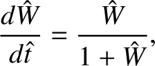$$\frac{d\hat{W}}{d\hat{t}} = \frac{\hat{W}}{1+\hat{W}},$$ (9.13)

which can be solved to give

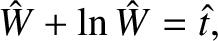$$\hat{W} + \ln\hat{W} = \hat{t},$$ (9.14)

assuming that $\hat{W}=0$ at $\hat{t}=-\infty$. Figure 9.1 shows the time evolution of the magnetic island width predicted by the previous equation. It can be seen that the evolution makes a smooth transition from exponential growth when $\hat{W}\ll 1$ (i.e., when the island width is much less than the linear layer width) to algebraic growth when $\hat{W}\gg 1$ (i.e., when the island width is much greater than the linear layer width).