Next: Electric dipole radiation
Up: Electromagnetic radiation
Previous: Introduction
The Hertzian dipole
Consider two small spherical conductors connected by a wire. Suppose that electric
charge flows periodically back and forth between the spheres. Let  be the instantaneous charge on
one of the conductors. The system has zero net charge, so
the charge on the other conductor is
be the instantaneous charge on
one of the conductors. The system has zero net charge, so
the charge on the other conductor is  . Let
. Let
 |
(1075) |
We expect the oscillating current flowing in the wire connecting the two spheres to
generate electromagnetic radiation (see Sect. 4.11). Let us consider the simple
case in which the length of the wire is small compared to the wave-length of the emitted
radiation. If this is the case, then the current  flowing between the conductors has the
same phase along the whole length of the wire. It follows that
flowing between the conductors has the
same phase along the whole length of the wire. It follows that
 |
(1076) |
where
 . This type of antenna is called a Hertzian dipole, after
the German physicist Heinrich Hertz.
. This type of antenna is called a Hertzian dipole, after
the German physicist Heinrich Hertz.
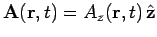
The magnetic vector potential generated by a current distribution
 is given by
the well-known formula (see Sect. 4.12)
is given by
the well-known formula (see Sect. 4.12)
![\begin{displaymath}
{\bf A}({\bf r}, t) = \frac{\mu_0}{4\pi} \int \frac{[{\bf j}]}{\vert{\bf r} - {\bf r}'\vert}
d^3{\bf r}',
\end{displaymath}](img2203.png) |
(1077) |
where
![\begin{displaymath}[f]= f({\bf r}', t - \vert{\bf r} - {\bf r}'\vert/c).
\end{displaymath}](img2204.png) |
(1078) |
Suppose that the wire is aligned along the  -axis, and extends from
  to
to  .
For a wire of negligible thickness, we can replace
.
For a wire of negligible thickness, we can replace
 by
by
 .
Thus,
.
Thus,
 , and
, and
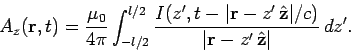 |
(1079) |
In the region  ,
,
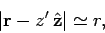 |
(1080) |
and
 |
(1081) |
The maximum error in the latter approximation is
 . This error (which is
a time) must be much less than a period of oscillation of the emitted radiation,
otherwise the phase of the radiation will be wrong. So
. This error (which is
a time) must be much less than a period of oscillation of the emitted radiation,
otherwise the phase of the radiation will be wrong. So
 |
(1082) |
which implies that  ,
where
,
where
 is the wave-length of the emitted radiation.
However,
we have already assumed that the length of the wire
is the wave-length of the emitted radiation.
However,
we have already assumed that the length of the wire  is much less than the wave-length of the
radiation, so the above inequality is automatically
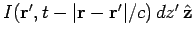
satisfied. Thus, in the far field region,
is much less than the wave-length of the
radiation, so the above inequality is automatically
satisfied. Thus, in the far field region,  , we can
write
, we can
write
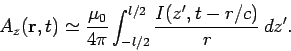 |
(1083) |
This integral is easy to perform, since the current is uniform along the length of the wire.
So,
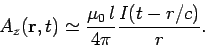 |
(1084) |
The scalar potential is most conveniently evaluated using the Lorentz gauge condition (see Sect. 4.12)
 |
(1085) |
Now,
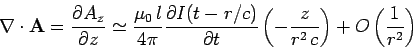 |
(1086) |
to leading order in  . Thus,
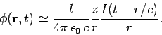 |
(1087) |
Given the vector and scalar potentials, Eqs. (1084) and (1087),
respectively, we can
evaluate the associated electric and magnetic fields using (see Sect. 4.12)
Note that we are only interested in radiation fields, which fall off like
with increasing distance from the source. It is easily demonstrated that
![\begin{displaymath}
{\bf E} \simeq - \frac{\omega l I_0}{4\pi \epsilon_0 \...
...rac{\sin[\omega (t-r/c)]}{r} \hat{\mbox{\boldmath$\theta$}},
\end{displaymath}](img2224.png) |
(1090) |
and
![\begin{displaymath}
{\bf B} \simeq -\frac{\omega l I_0 }{4\pi \epsilon_0 \...
...c{\sin
[\omega (t-r/c)]}{r} \hat{\mbox{\boldmath$\varphi$}}.
\end{displaymath}](img2225.png) |
(1091) |
Here, ( ,
,  ,
,  ) are standard spherical polar coordinates aligned along
the -axis. The above expressions for the far field (i.e., )
electromagnetic fields generated by a localized oscillating current are also
easily derived from Eqs. (552) and (553). Note that the fields are symmetric in
the azimuthal angle . There is no radiation along the axis of the oscillating
dipole (i.e.,
) are standard spherical polar coordinates aligned along
the -axis. The above expressions for the far field (i.e., )
electromagnetic fields generated by a localized oscillating current are also
easily derived from Eqs. (552) and (553). Note that the fields are symmetric in
the azimuthal angle . There is no radiation along the axis of the oscillating
dipole (i.e.,  ), and the maximum emission is in the plane perpendicular
to this axis (i.e.,
), and the maximum emission is in the plane perpendicular
to this axis (i.e.,
 ).
).
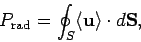
The average power crossing a spherical surface  (whose radius is much greater than
 ) is
) is
 |
(1092) |
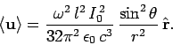
where the average is over a single period of oscillation of the wave, and
the Poynting flux is given by (see Sect. 8.2)
![\begin{displaymath}
{\bf u} = \frac{ {\bf E} \times{\bf B}}{\mu_0} = \frac{\omeg...
...sin^2[\omega(t-r/c)] \frac{\sin^2\theta}{r^2}
\hat{\bf r}.
\end{displaymath}](img2229.png) |
(1093) |
It follows that
 |
(1094) |
Note that the energy flux is radially outwards from the source. The total power
flux across is given by
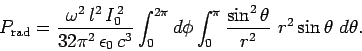 |
(1095) |
Thus,
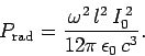 |
(1096) |
The total flux is independent of the radius of , as is to be expected if
energy is conserved.
Recall that for a resistor of resistance  the average ohmic heating power is
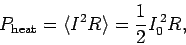 |
(1097) |
assuming that
 . It is convenient to define the radiation
resistance of a Hertzian dipole antenna:
. It is convenient to define the radiation
resistance of a Hertzian dipole antenna:
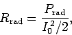 |
(1098) |
so that
 |
(1099) |
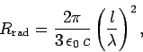
where
is the wave-length of the radiation.
In fact,
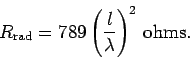 |
(1100) |
In the theory
of electrical circuits, an antenna is conventionally represented as
a resistor whose resistance is equal
to the characteristic radiation resistance of the antenna plus its real
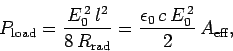
resistance. The power loss
 associated with the radiation resistance
is due to the emission of electromagnetic radiation. The power loss
associated with the radiation resistance
is due to the emission of electromagnetic radiation. The power loss
 associated with
the real resistance is
due to ohmic heating of the antenna.
associated with
the real resistance is
due to ohmic heating of the antenna.
Note that the formula (1100) is only valid for . This suggests
that
 for most Hertzian
dipole antennas: i.e., the radiated power is
swamped by the ohmic losses. Thus, antennas whose lengths are much less than
that of the emitted radiation tend to be extremely inefficient.
In fact, it is necessary
to have
for most Hertzian
dipole antennas: i.e., the radiated power is
swamped by the ohmic losses. Thus, antennas whose lengths are much less than
that of the emitted radiation tend to be extremely inefficient.
In fact, it is necessary
to have  in order to obtain an efficient antenna. The simplest
practical antenna is the half-wave antenna, for which
in order to obtain an efficient antenna. The simplest
practical antenna is the half-wave antenna, for which  . This
can be analyzed as a series of Hertzian dipole antennas
stacked on top of one another, each
slightly out of phase with its neighbours. The characteristic radiation resistance
of a half-wave antenna is
. This
can be analyzed as a series of Hertzian dipole antennas
stacked on top of one another, each
slightly out of phase with its neighbours. The characteristic radiation resistance
of a half-wave antenna is
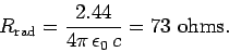 |
(1101) |
Antennas can also be used to receive electromagnetic radiation. The incoming wave
induces a voltage in the antenna, which can be detected in an electrical
circuit
connected to the antenna. In fact, this process is equivalent to the emission
of electromagnetic waves by the antenna viewed in reverse. It
is easily demonstrated that antennas most readily detect electromagnetic radiation
incident from those directions in which they preferentially emit radiation.
Thus, a Hertzian dipole antenna is unable to detect radiation incident along
its axis, and most efficiently detects radiation incident in the plane perpendicular
to this axis. In the theory of electrical circuits, a receiving antenna is represented
as a voltage source in series with a resistor. The voltage source,
 , represents
the voltage induced in the antenna by the incoming wave. The resistor,
, represents
the voltage induced in the antenna by the incoming wave. The resistor,
 , represents the power re-radiated by the antenna (here,
the real resistance
of the antenna is neglected). Let us represent the detector circuit as a single
load resistor
, represents the power re-radiated by the antenna (here,
the real resistance
of the antenna is neglected). Let us represent the detector circuit as a single
load resistor  , connected in series with the antenna. The question is:
how can we choose so that the maximum power is extracted from the
wave and transmitted to the load resistor? According to Ohm's law:
, connected in series with the antenna. The question is:
how can we choose so that the maximum power is extracted from the
wave and transmitted to the load resistor? According to Ohm's law:
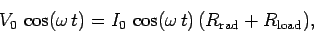 |
(1102) |
where
is the current induced in the circuit.
The power input to the circuit is
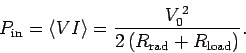 |
(1103) |
The power transferred to the load is
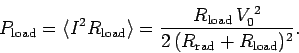 |
(1104) |
The power re-radiated by the antenna is
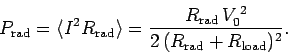 |
(1105) |
Note that
 .
The maximum power transfer to the load occurs when
.
The maximum power transfer to the load occurs when
![\begin{displaymath}
\frac{\partial P_{\rm load}}{\partial R_{\rm load}} = \frac{...
...d} - R_{\rm load}}{(R_{\rm rad} + R_{\rm load})^3}\right] = 0.
\end{displaymath}](img2251.png) |
(1106) |
Thus, the maximum transfer rate corresponds to
 |
(1107) |
In other words, the resistance of the load circuit must match the radiation
resistance of the antenna.
For this optimum case,
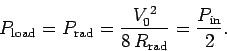 |
(1108) |
So, in the optimum case half
of the power absorbed by the antenna is immediately
re-radiated. Clearly, an antenna which
is receiving electromagnetic radiation is also emitting it.
This is how the BBC catch people who do not pay their television license fee in
England. They have vans which can detect the radiation emitted by
a TV aerial whilst it is in use (they can even tell which channel you are watching!).
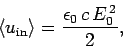
For a Hertzian dipole antenna interacting with an incoming wave whose electric
field has an amplitude  , we expect
 |
(1109) |
Here, we have used the fact that the wave-length of the radiation is much longer
than the length of the antenna. We have also assumed that the antenna is
properly aligned (i.e., the radiation is incident perpendicular to the axis of the
antenna). The Poynting flux of the incoming wave is [see Eq. (1052)]
 |
(1110) |
whereas the power transferred to a properly matched detector circuit is
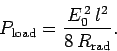 |
(1111) |
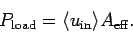
Consider an idealized antenna in which all
incoming radiation incident on some area  is absorbed, and then
magically transferred to the detector circuit, with no re-radiation.
Suppose that the power absorbed from the idealized antenna
matches that absorbed from
the
real antenna. This implies that
is absorbed, and then
magically transferred to the detector circuit, with no re-radiation.
Suppose that the power absorbed from the idealized antenna
matches that absorbed from
the
real antenna. This implies that
 |
(1112) |
The quantity is called the effective area of the antenna: it is
the area of the idealized antenna which absorbs as much net power from the incoming
wave as the actual antenna.
Thus,
 |
(1113) |
giving
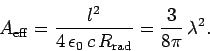 |
(1114) |
It is clear that the effective area of a Hertzian dipole antenna is of
order the wave-length squared of the incoming radiation.
For a properly aligned half-wave antenna,
 |
(1115) |
Thus, the antenna, which is essentially one-dimensional with length  ,
acts as if it is two-dimensional, with width
,
acts as if it is two-dimensional, with width  , as far as its
absorption of incoming electromagnetic radiation is concerned.
, as far as its
absorption of incoming electromagnetic radiation is concerned.
Next: Electric dipole radiation
Up: Electromagnetic radiation
Previous: Introduction
Richard Fitzpatrick
2006-02-02