Retarded fields

We know the solution to Maxwell's equations in terms of retarded potentials. Let us now construct the associated electric and magnetic fields using

$${\bf E} = - \nabla\phi - \frac{\partial {\bf A}}{\partial t},$$ (533)

$${\bf B} = \nabla\times{\bf A}.$$ (534)

It is helpful to write

$${\bf R} = {\bf r} - {\bf r}',$$ (535)

where 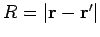$R = \vert{\bf r} - {\bf r}'\vert$. The retarded time becomes 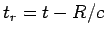$t_r = t- R/c$, and a general retarded quantity is written $[F({\bf r}, t)]\equiv F({\bf r}, t_r)$. Thus, we can write the retarded potential solutions of Maxwell's equations in the especially compact form:

$$\phi = \frac{1}{4\pi \epsilon_0} \int \frac{[\rho]}{R} dV',$$ (536)

$${\bf A} = \frac{\mu_0}{4\pi} \int \frac{[{\bf j}]}{R} dV',$$ (537)

where $dV' \equiv d^3{\bf r}'$.

It is easily seen that

$$\nabla\phi = \frac{1}{4\pi \epsilon_0}\int \left( [\rho] \nabla(R^{-1}) + \frac{[\partial\rho/\partial t]}{R} \nabla t_r\right) dV'$$

$$= - \frac{1}{4\pi\epsilon_0} \int \left( \frac{[\rho]}{R^3} {\bf R} + \frac{[\partial\rho/\partial t]}{cR^2} {\bf R} \right) dV',$$ (538)

where use has been made of

$$\nabla R = \frac{\bf R}{R},   \nabla( R^{-1})= - \frac{\bf R}{R^3},   \nabla t_r = - \frac{\bf R}{cR}.$$ (539)

Likewise,

$$\nabla\times{\bf A} = \frac{\mu_0}{4\pi} \int \left( \nabla(R^{-1}) \times [{\bf j}] + \frac{\nabla t_r\times [\partial {\bf j}/\partial t]}{R} \right) dV'$$

$$= -\frac{\mu_0}{4\pi} \int \left( \frac{{\bf R} \times [{\bf j}]}{R^3} + \frac{{\bf R} \times [\partial {\bf j}/\partial t]}{cR^2} \right) dV'.$$ (540)

Equations (533), (534), (538), and (540) can be combined to give

$${\bf E} = \frac{1}{4\pi \epsilon_0} \int \left( [\rho] \f... ...2} - \frac{[\partial {\bf j}/\partial t]}{c^2 R} \right) dV',$$ (541)

which is the time-dependent generalization of Coulomb's law, and

$${\bf B} = \frac{\mu_0}{4\pi} \int \left( \frac{ [{\bf j}]\ti... ...rtial {\bf j}/\partial t]\times {\bf R} } {cR^2} \right) dV',$$ (542)

which is the time-dependent generalization of the Biot-Savart law.

Suppose that the typical variation time-scale of our charges and currents is $t_0$. Let us define $R_0 = c t_0$, which is the distance a light ray travels in time $t_0$. We can evaluate Eqs. (541) and (542) in two asymptotic limits: the near field region $R\ll R_0$, and the far field region $R\gg R_0$. In the near field region

$$\frac{\vert t -t_r\vert}{t_0} = \frac{R}{R_0} \ll 1,$$ (543)

so the difference between retarded time and standard time is relatively small. This allows us to expand retarded quantities in a Taylor series. Thus,

$$[\rho]\simeq \rho + \frac{\partial\rho}{\partial t} (t_r-t)... ...}{2} \frac{\partial^2 \rho}{\partial t^2} (t_r -t )^2+\cdots,$$ (544)

giving

$$[\rho]\simeq \rho - \frac{\partial \rho}{\partial t} \frac{R}... ...\frac{\partial^2 \rho}{\partial t^2} \frac{R^2}{c^2} + \cdots.$$ (545)

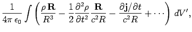
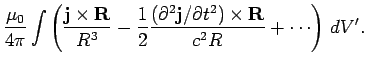
Expansion of the retarded quantities in the near field region yields

$${\bf E} \simeq \frac{1}{4\pi \epsilon_0} \int \left( \frac{\rho {\bf R}}{R^3}... ...c{\bf R}{c^2 R} - \frac{\partial {\bf j}/\partial t}{c^2 R}+\cdots\right) dV',$$ (546)

$${\bf B} \simeq \frac{\mu_0}{4\pi} \int \left(\frac{{\bf j}\times{\bf R}}{R^3} - ... ...{(\partial^2 {\bf j}/ \partial t^2)\times{\bf R}}{c^2 R} +\cdots \right) d V'.$$ (547)

In Eq. (546), the first term on the right-hand side corresponds to Coulomb's law, the second term is the correction due to retardation effects, and the third term corresponds to Faraday induction. In Eq. (547), the first term on the right-hand side is the Biot-Savart law, and the second term is the correction due to retardation effects. Note that the retardation corrections are only of order $(R/R_0)^2$. We might suppose, from looking at Eqs. (541) and (542), that the corrections should be of order $R/R_0$. However, all of the order $R/R_0$ terms canceled out in the previous expansion. Suppose, then, that we have a d.c. circuit sitting on a laboratory benchtop. Let the currents in the circuit change on a typical time-scale of one tenth of a second. In this time, light can travel about $3\times 10^7$ meters, so $R_0 \sim 30,000$ kilometers. The length-scale of the experiment is about one meter, so $R = 1$ meter. Thus, the retardation corrections are of order $(3\times 10^7)^{-2} \sim 10^{-15}$. It is clear that we are fairly safe just using Coulomb's law, Faraday's law, and the Biot-Savart law to analyze the fields generated by this type of circuit.

In the far field region, $R\gg R_0$, Eqs. (541) and (542) are dominated by the terms which vary like $R^{-1}$, so

$${\bf E} \simeq -\frac{1}{4\pi \epsilon_0}\int\frac{[\partial {\bf j}_\perp /\partial t]}{c^2 R} dV',$$ (548)

$${\bf B} \simeq \frac{\mu_0}{4\pi} \int \frac{ [\partial {\bf j}_\perp/\partial t]\times {\bf R} } {c R^2} dV',$$ (549)

where

$${\bf j}_\perp = {\bf j} - \frac{({\bf j} \cdot {\bf R})}{R^2} {\bf R}.$$ (550)

Here, use has been made of $[\partial \rho/\partial t] = -[\nabla\cdot {\bf j}]$ and $[\nabla\cdot {\bf j} ] = -[\partial {\bf j}/\partial t]\cdot {\bf R}/c R + O(1/R^2)$. Suppose that our charges and currents are localized to some region in the vicinity of ${\bf r}' = {\bf r}_\ast$. Let ${\bf R_\ast} = {\bf r} - {\bf r}_\ast$, with $R_\ast = \vert{\bf r} - {\bf r}_\ast\vert$. Suppose that the extent of the current and charge containing region is much less than $R_\ast$. It follows that retarded quantities can be written

$$[ \rho({\bf r}, t)]\simeq \rho({\bf r}, t - R_\ast/c),$$ (551)

etc. Thus, the electric field reduces to

$${\bf E} \simeq -\frac{1}{4\pi \epsilon_0} \frac{\left[ \int \partial {\bf j}_\perp/\partial t dV'\right]}{c^2 R_\ast},$$ (552)

whereas the magnetic field is given by

$${\bf B} \simeq \frac{1}{4\pi \epsilon_0} \frac{ \left[ \int... ...partial t dV'\right] \times{\bf R}_\ast }{c^3 R_\ast^{ 2}}.$$ (553)

Note that

$$\frac{E}{B} = c,$$ (554)

and

$${\bf E} \cdot {\bf B} = 0.$$ (555)

This configuration of electric and magnetic fields is characteristic of an electromagnetic wave (see Sect. 4.7). Thus, Eqs. (552) and (553) describe an electromagnetic wave propagating radially away from the charge and current containing region. Note that the wave is driven by time-varying electric currents. Now, charges moving with a constant velocity constitute a steady current, so a non-steady current is associated with accelerating charges. We conclude that accelerating electric charges emit electromagnetic waves. The wave fields, (552) and (553), fall off like the inverse of the distance from the wave source. This behaviour should be contrasted with that of Coulomb or Biot-Savart fields, which fall off like the inverse square of the distance from the source. The fact that wave fields attenuate fairly gently with increasing distance from the source is what makes astronomy possible. If wave fields obeyed an inverse square law then no appreciable radiation would reach us from the rest of the Universe.

In conclusion, electric and magnetic fields look simple in the near field region (they are just Coulomb fields, etc.) and also in the far field region (they are just electromagnetic waves). Only in the intermediate region, $R\sim R_0$, do things start getting really complicated (so we generally do not look in this region!).