Advanced potentials?

We have defined the retarded time

$$t_r = t - \vert{\bf r} - {\bf r}'\vert/c$$ (522)

as the latest time at which a light signal emitted from position ${\bf r}'$ would reach position ${\bf r}$ before time $t$. We have also shown that a solution to Maxwell's equations can be written in terms of retarded potentials:

$$\phi({\bf r}, t) = \frac{1}{4\pi \epsilon_0} \int \frac{ \rho({\bf r}', t_r)}{\vert{\bf r} - {\bf r}'\vert} d^3{\bf r}',$$ (523)

etc. But, is this the most general solution? Suppose that we define the advanced time.

$$t_a = t + \vert{\bf r} - {\bf r}'\vert/c.$$ (524)

This is the time a light signal emitted at time $t$ from position ${\bf r}$ would reach position ${\bf r}'$. It turns out that we can also write a solution to Maxwell's equations in terms of advanced potentials:

$$\phi({\bf r}, t) = \frac{1}{4\pi \epsilon_0} \int \frac{ \rho({\bf r}', t_a)}{\vert{\bf r} - {\bf r}'\vert} d^3{\bf r}',$$ (525)

etc. In fact, this is just as good a solution to Maxwell's equation as the one involving retarded potentials. To get some idea what is going on, let us examine the Green's function corresponding to our retarded potential solution:

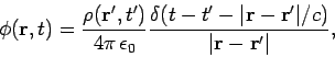$$\phi({\bf r}, t) = \frac{\rho({\bf r}' ,t ')} {4\pi \epsil... ...vert{\bf r} - {\bf r}'\vert/c)}{\vert{\bf r} - {\bf r}'\vert},$$ (526)

with a similar equation for the vector potential. This says that the charge density present at position ${\bf r}'$ and time $t'$ emits a spherical wave in the scalar potential which propagates forwards in time. The Green's function corresponding to our advanced potential solution is

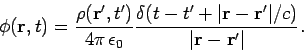$$\phi({\bf r}, t) = \frac{\rho({\bf r}' ,t ')} {4\pi \epsil... ...vert{\bf r} - {\bf r}'\vert/c)}{\vert{\bf r} - {\bf r}'\vert}.$$ (527)

This says that the charge density present at position ${\bf r}'$ and time $t'$ emits a spherical wave in the scalar potential which propagates backwards in time. ``But, hang on a minute,'' you might say, ``everybody knows that electromagnetic waves can't travel backwards in time. If they did then causality would be violated.'' Well, you know that electromagnetic waves do not propagate backwards in time, I know that electromagnetic waves do not propagate backwards in time, but the question is do Maxwell's equations know this? Consider the wave equation for the scalar potential:

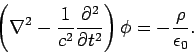$$\left( \nabla^2 - \frac{1}{c^2} \frac{\partial^2 }{\partial t^2}\right) \phi = -\frac{\rho} {\epsilon_0}.$$ (528)

This equation is manifestly symmetric in time (i.e., it is invariant under the transformation $t\rightarrow -t$). Thus, backward traveling waves are just as good a solution to this equation as forward traveling waves. The equation is also symmetric in space (i.e., it is invariant under the transformation $x\rightarrow -x$). So, why do we adopt the Green's function (526) which is symmetric in space (i.e., it is invariant under $x\rightarrow -x$) but asymmetric in time (i.e., it is not invariant under $t\rightarrow -t$)? Would it not be better to use the completely symmetric Green's function

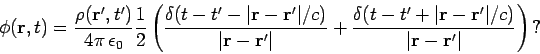$$\phi({\bf r}, t) = \frac{\rho({\bf r}' ,t ')} {4\pi \epsil... ...r} - {\bf r}'\vert/c)}{\vert{\bf r} - {\bf r}'\vert}\right) ?$$ (529)

In other words, a charge emits half of its waves running forwards in time (i.e., retarded waves), and the other half running backwards in time (i.e., advanced waves). This sounds completely crazy! However, in the 1940's Richard P. Feynman and John A. Wheeler pointed out that under certain circumstances this prescription gives the right answer. Consider a charge interacting with ``the rest of the Universe,'' where the ``rest of the Universe'' denotes all of the distant charges in the Universe, and is, by implication, an awful long way away from our original charge. Suppose that the ``rest of the Universe'' is a perfect reflector of advanced waves and a perfect absorbed of retarded waves. The waves emitted by the charge can be written schematically as

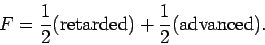$$F = \frac{1}{2} ({\rm retarded}) + \frac{1}{2} ({\rm advanced}).$$ (530)

The response of the rest of the universe is written

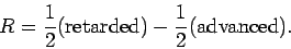$$R = \frac{1}{2} ({\rm retarded}) - \frac{1}{2} ({\rm advanced}).$$ (531)

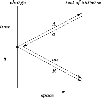
This is illustrated in the space-time diagram Fig. 40. Here, $A$ and $R$ denote the advanced and retarded waves emitted by the charge, respectively. The advanced wave travels to ``the rest of the Universe'' and is reflected: i.e., the distant charges oscillate in response to the advanced wave and emit a retarded wave $a$, as shown. The retarded wave $a$ is spherical wave which converges on the original charge, passes through the charge, and then diverges again. The divergent wave is denoted $aa$. Note that $a$ looks like a negative advanced wave emitted by the charge, whereas $aa$ looks like a positive retarded wave emitted by the charge. This is essentially what Eq. (531) says. The retarded waves $R$ and $aa$ are absorbed by ``the rest of the Universe.''

Figure 40:

If we add the waves emitted by the charge to the response of ``the rest of the Universe'' we obtain

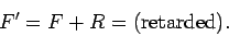$$F' = F+R = ({\rm retarded}).$$ (532)

Thus, charges appear to emit only retarded waves, which agrees with our everyday experience. Clearly, in this model we have side-stepped the problem of a time asymmetric Green's function by adopting time asymmetric boundary conditions to the Universe: i.e., the distant charges in the Universe absorb retarded waves and reflect advanced waves. This is possible because the absorption takes place at the end of the Universe (i.e., at the ``big crunch,'' or whatever) and the reflection takes place at the beginning of the Universe (i.e., at the ``big bang''). It is quite plausible that the state of the Universe (and, hence, its interaction with electromagnetic waves) is completely different at these two times. It should be pointed out that the Feynman-Wheeler model runs into trouble when one tries to combine electromagnetism with quantum mechanics. These difficulties have yet to be resolved, so at present the status of this model is that it is ``an interesting idea,'' but it is still not fully accepted into the canon of physics.