Gravitational Potential of Uniform Spheroid
Let us use Poisson's equation, (1.273), to calculate
the gravitational potential generated around a spheroid
of uniform mass density  and mean radius
  . A spheroid is
the solid body produced by rotating an ellipse about a major or
a minor axis. Let the center of the spheroid be located at the origin, let its axis of rotation coincide with the
. A spheroid is
the solid body produced by rotating an ellipse about a major or
a minor axis. Let the center of the spheroid be located at the origin, let its axis of rotation coincide with the  -axis,
and let its outer boundary satisfy
-axis,
and let its outer boundary satisfy
![$\displaystyle r = R_\theta(\theta) = R\left[1-\frac{2}{3}\,\epsilon\,P_2(\cos\theta)\right],$](img805.png) |
(1.328) |
where  is termed the ellipticity. Here,
  ,
,  ,
,  are conventional spherical coordinates. (See Section A.23.)
Moreover,
are conventional spherical coordinates. (See Section A.23.)
Moreover,
 |
(1.329) |
is a Legendre polynomial of degree 2.
It can be seen that the radius of the
spheroid at the poles (i.e., along the rotation axis,  ) is
) is
 , whereas
the radius at the equator (i.e., in the bisecting plane perpendicular to the axis,
, whereas
the radius at the equator (i.e., in the bisecting plane perpendicular to the axis,
 ) is
) is
 . Hence,
 |
(1.330) |
Let us assume that
 , so that the spheroid is very close to being a
sphere. If
, so that the spheroid is very close to being a
sphere. If
 then the spheroid is
slightly squashed along its axis of rotation, and is termed oblate. Likewise, if
then the spheroid is
slightly squashed along its axis of rotation, and is termed oblate. Likewise, if
 then the spheroid is slightly elongated along its axis, and is
termed prolate. See Figure 1.18.
Of course, if
then the spheroid is slightly elongated along its axis, and is
termed prolate. See Figure 1.18.
Of course, if
 then the spheroid reduces to a sphere. Note that is the surface-averaged radius of the
spheroid, which implies that the volume of the spheroid is equal to that of a sphere of radius . In other words, the
slight squashing or elongation of the spheroid along its axis, as is varied, does not modify its volume.
then the spheroid reduces to a sphere. Note that is the surface-averaged radius of the
spheroid, which implies that the volume of the spheroid is equal to that of a sphere of radius . In other words, the
slight squashing or elongation of the spheroid along its axis, as is varied, does not modify its volume.
Figure 1.18:
Prolate and oblate spheroids.
|
|
Let
 and
and
 be the gravitational potential and the mass density of the
spheroid, respectively.
Let us write
be the gravitational potential and the mass density of the
spheroid, respectively.
Let us write
 |
(1.331) |
and
 |
(1.332) |
where
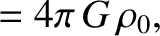
![$\displaystyle \rho_0(r) =\left\{\begin{array}{lll}\gamma&~~~~&r\leq R\\ [0.5ex]0&&r>R\end{array}\right.,$](img822.png) |
(1.333) |
and
 |
(1.334) |
Here,  is a Dirac delta function. (See Section 2.1.6.) This function has the unusual property that
 for
for  ,
,
 at
at  , but
, but
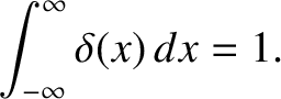 |
(1.335) |
Thus, a Dirac delta function is an integrable spike function, centered on , that has unit area under it.
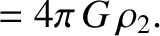
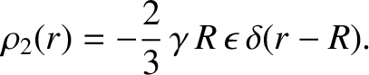
Note that  is the density distribution of a uniform sphere of density and radius .
On the other hand,
is the density distribution of a uniform sphere of density and radius .
On the other hand,
![$\rho_2(r)\,P_2(\cos\theta)=\gamma\,[R_\theta(\theta)-R]\,\delta(r-R)$](img830.png) is the density distribution obtained by taking the slight excess or deficit of surface
mass, due to the deviation from sphericity of the spheroid, and placing it all at radius . Note that, in writing Equation (1.331), we have assumed that an axisymmetric mass distribution (i.e., a distribution that is
independent of the azimuthal angle, ) gives rise to an axisymmetric gravitational potential.
is the density distribution obtained by taking the slight excess or deficit of surface
mass, due to the deviation from sphericity of the spheroid, and placing it all at radius . Note that, in writing Equation (1.331), we have assumed that an axisymmetric mass distribution (i.e., a distribution that is
independent of the azimuthal angle, ) gives rise to an axisymmetric gravitational potential.
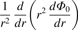
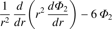
Now, in spherical coordinates, the Laplacian of
(i.e., a function of spherical coordinates that is independent of the
azimuthal angle, ) takes the form
![$\displaystyle \frac{1}{r^2}\,\frac{\partial}{\partial r}\!\left(r^2\,\frac{\par...
...}{\partial\mu}\!\left[(1-\mu^2)\,\frac{\partial{\mit\Phi}}{\partial\mu}\right],$](img831.png) |
(1.336) |
where
 . (See Section A.23.) Thus, according to Poisson's equation, (1.273), we can write
Here, we have made use of the easily proved result
. (See Section A.23.) Thus, according to Poisson's equation, (1.273), we can write
Here, we have made use of the easily proved result
![$\displaystyle \frac{d}{d\mu}\!\left[(1-\mu^2)\,\frac{dP_2(\mu)}{d\mu}\right]= -6\,P_2(\mu).$](img837.png) |
(1.339) |
We have also employed the readily demonstrated result that
 |
(1.340) |
which allows us to separately equate the components of Poisson's equation that are independent of , and
that vary with as
 .
.
Equations (1.333) and (1.337) must be solved subject to the physical boundary conditions that
 be finite at both
  and
and  , and that
and its first derivative both
be continuous at
, and that
and its first derivative both
be continuous at  . The latter constraint ensures that the gravitational acceleration is both finite and
continuous at . It is easily seen, by inspection, that the appropriate solution is
. The latter constraint ensures that the gravitational acceleration is both finite and
continuous at . It is easily seen, by inspection, that the appropriate solution is
![$\displaystyle {\mit\Phi}_0(r) = \frac{G\,M}{2\,R}\left[\left(\frac{r}{R}\right)^2-3\right]$](img844.png) |
(1.341) |
for  , and
, and
 |
(1.342) |
for  . Here,
 is the mass of the spheroid.
If we calculate the associated gravitational acceleration,
is the mass of the spheroid.
If we calculate the associated gravitational acceleration,
 , then we
can see that this solution is the same as that found for a uniform sphere in Section 1.8.3 using Gauss's law.
, then we
can see that this solution is the same as that found for a uniform sphere in Section 1.8.3 using Gauss's law.
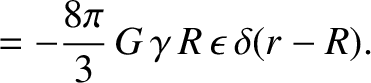
Equation (1.334) and (1.338) yield
Now,
 must be continuous across otherwise the gravitational acceleration would be infinite.
Hence, integrating the previous equation across , and making use of Equation (1.335), we obtain
must be continuous across otherwise the gravitational acceleration would be infinite.
Hence, integrating the previous equation across , and making use of Equation (1.335), we obtain
![$\displaystyle \left[\frac{d{\mit\Phi}_2}{dr}\right]_{r=R-}^{r=R+} = - \frac{8\pi}{3}\,G\,\gamma\,R\,\epsilon.$](img850.png) |
(1.344) |
Note that the discontinuity in the gradient of
 at is just an artifact of the fact that we have
placed all of the excess or deficit of surface
mass at this radius, and is not a real phenomenon (i.e., the discontinuity would be resolved if we were to spread the mass out slightly).
Now, for
at is just an artifact of the fact that we have
placed all of the excess or deficit of surface
mass at this radius, and is not a real phenomenon (i.e., the discontinuity would be resolved if we were to spread the mass out slightly).
Now, for  , the Dirac delta function,
 , is zero, and Equation (1.343) reduces to
 |
 |
(1.345) |
 |
(1.346) |
for , and
 |
(1.347) |
for .
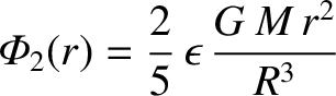
Hence, we deduce that the net gravitational potential is
![$\displaystyle {\mit\Phi}(r,\theta)= \frac{G\,M}{2\,R}\left[\left(\frac{r}{R}\right)^2-3\right] +\frac{2}{5}\,\epsilon\,\frac{G\,M\,r^2}{R^3}\,P_2(\cos\theta)$](img857.png) |
(1.348) |
inside the spheroid, and
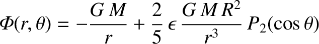 |
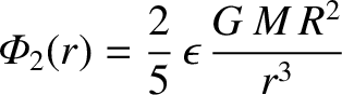
(1.349) |
outside the spheroid. In particular, the gravitational potential on the surface of the spheroid is
![$\displaystyle {\mit\Phi}(R_\theta,\theta)= -\frac{G\,M}{R}\left[1+\frac{4}{15}\,\epsilon\,P_2(\cos\theta)+{\cal O}(\epsilon^2)\right].$](img859.png) |
(1.350) |
![\includegraphics[height=2.25in]{Chapter02/fig12_01.eps}](img817.png)