Next: Quantum Mechanics Up: Relativity and Electromagnetism Previous: Transformation of Electromagnetic Fields
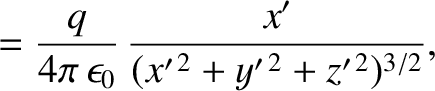
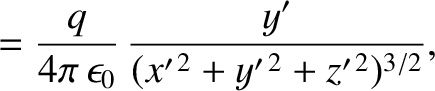
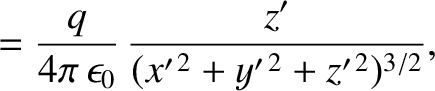
 , that is at rest at the origin of an inertial reference frame
  . The electric
and magnetic fields generated by the charge at displacement
. The electric
and magnetic fields generated by the charge at displacement  in frame are
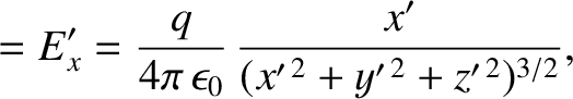
 |
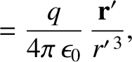 |
(3.286) |
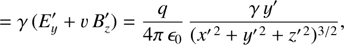
 |
 |
(3.287) |
 |
 |
(3.288) |
 |
 |
(3.289) |
 |
 |
(3.290) |
 |
 |
(3.291) |
Let us transform to an inertial reference frame,  , that is in a standard configuration, and moves with
velocity
, that is in a standard configuration, and moves with
velocity
 , with respect to frame . Thus, in frame , the charge appears to move with
velocity
, with respect to frame . Thus, in frame , the charge appears to move with
velocity
 . Making use of the field transformation relations, (3.278)–(3.283),
with primed and unprimed fields swapped, and
. Making use of the field transformation relations, (3.278)–(3.283),
with primed and unprimed fields swapped, and
 , we obtain
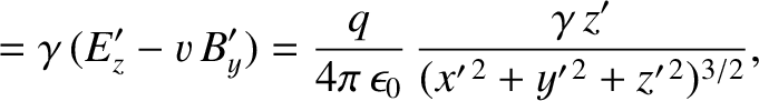
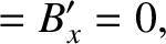
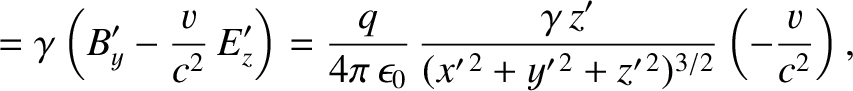
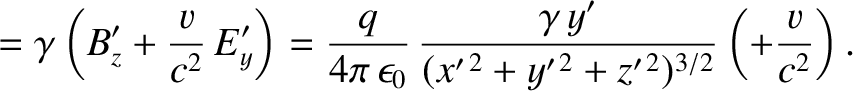
Consider the electric and magnetic fields generated by the charge at some point  in frame whose displacement is
 ,
,  . See Figure 3.18. The displacement of the charge in frame is
 0, 0). Let
 |
(3.298) |
to point . A Lorentz transformation (see Section 3.2.7) between frames and reveals that
Let us write
 |
 |
(3.302) |
 |
 |
(3.303) |
 |
 |
(3.304) |
 is the angle subtended between
  and
and  , and
, and  is an
azimuthal angle. See Figure 3.18. It is easily demonstrated from the previous six equations that
is an
azimuthal angle. See Figure 3.18. It is easily demonstrated from the previous six equations that
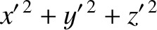 |
 |
|
![$\displaystyle = \left(\gamma^2\,\cos^2\theta + \sin^2\theta\right)s^2=\left[(\gamma^2-1)\,\cos^2\theta+1\right]s^2$](img2861.png) |
||
 |
(3.305) |
 is the component of that is directed from the instantaneous position of the charge to the point .
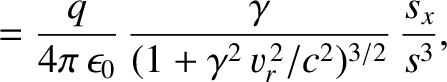
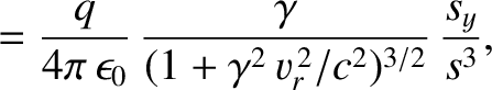
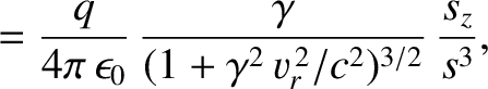
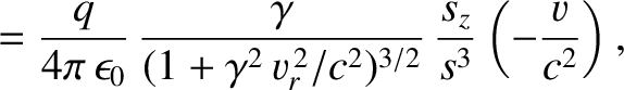
Thus, making use of Equations (3.292)–(3.297) and Equations (3.299)–(3.301), we obtain
is the component of that is directed from the instantaneous position of the charge to the point .
Thus, making use of Equations (3.292)–(3.297) and Equations (3.299)–(3.301), we obtain
 |
 |
(3.306) |
 |
 |
(3.307) |
 |
 |
(3.308) |
 |
 |
(3.309) |
 |
 |
(3.310) |
 |
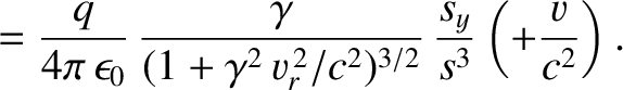 |
(3.311) |
Note that the electric field-lines generated by a moving electric charge are straight-lines that are directed from the
instantaneous position of the charge to the point of observation. At low velocities (i.e.,  ), the field-lines are
equally spaced around the charge. However, as
), the field-lines are
equally spaced around the charge. However, as
 , the field-lines become increasingly bunched in the plane
transverse to the charge's direction of motion that passes through the charge. This is illustrated schematically in Figure 3.19. The magnetic field generated by a moving charge is
, the field-lines become increasingly bunched in the plane
transverse to the charge's direction of motion that passes through the charge. This is illustrated schematically in Figure 3.19. The magnetic field generated by a moving charge is
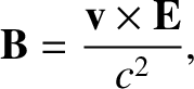 |
(3.312) |
is the charge's velocity, and  is the electric field generated by the charge.
![\includegraphics[height=2.5in]{Chapter04/theta.eps}](img2844.png)


![\includegraphics[height=2.75in]{Chapter04/charge.eps}](img2869.png)