


Next: Boundary Layer on a
Up: Incompressible Boundary Layers
Previous: Boundary Layer Equations
Self-Similar Boundary Layers
The boundary layer equation, (8.35), takes the form of a nonlinear partial
differential equation that is extremely difficult to solve exactly. However, considerable progress can be made if
this equation is converted into an ordinary differential equation by demanding that its solutions be
self-similar. Self-similar solutions are such that, at a given distance,  , along the layer, the tangential flow profile,
  , is
a scaled version of some common profile: that is,
, is
a scaled version of some common profile: that is,
![$ v_x(x,y)= U(x)\,F[y/\delta(x)]$](img2914.png) , where
, where  is a scale-factor, and
  a dimensionless function. It follows that
![$ \psi(x,y)=-U(x)\,\delta(x)\,f[y/\delta(x)]$](img2916.png) , where
, where
 .
.
Let us search for a self-similar solution to Equation (8.35) of the general form
![$\displaystyle \psi(x,y) = -\left[\frac{2\,\nu\,U_0\,x^{\,m+1}}{m+1}\right]^{1/2...
...)=-U_0\,x^{\,m}\left[\frac{2\,\nu}{(m+1)\,U_0\,x^{\,m-1}}\right]^{1/2} f(\eta),$](img2918.png) |
(8.41) |
where
![$\displaystyle \eta =\left[\frac{(m+1)\,U_0\,x^{\,m-1}}{2\,\nu}\right]^{1/2}y.$](img2919.png) |
(8.42) |
This implies that
![$ \delta(x)=[2\,\nu/(m+1)\,U_0\,x^{\,m-1}]^{1/2}$](img2920.png) , and
, and
 .
Here,
.
Here,  and
and  are constants. Moreover,
 has dimensions of velocity, whereas
,
has dimensions of velocity, whereas
,  , and
, and  , are dimensionless.
Transforming variables from
,
, are dimensionless.
Transforming variables from
,  to
,
, we find that
to
,
, we find that
Hence,
 |
![$\displaystyle = -\left[\frac{\nu\,U_0\,x^{\,m-1}}{2\,(m+1)}\right]^{1/2}[(m+1)\,f+(m-1)\,\eta\,f'],$](img2927.png) |
(8.45) |
 |
 |
(8.46) |
 |
![$\displaystyle =-\left[\frac{(m+1)\,U_0^{\,3}\,x^{\,3\,m-1}}{2\,\nu}\right]^{1/2}f'',$](img2931.png) |
(8.47) |
 |
![$\displaystyle = -\frac{U_0\,x^{\,m-1}}{2}\,[2\,m\,f'+(m-1)\,\eta\,f''],$](img2933.png) |
(8.48) |
 |
 |
(8.49) |
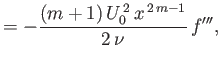
where
 . Thus, Equation (8.35)
becomes
. Thus, Equation (8.35)
becomes
 |
(8.50) |
Because the left-hand side of the previous equation is a (non-constant) function of
, while the right-hand side
is a function of
(and as
and
are independent variables), the equation can only be satisfied if its right-hand
side takes a constant value. In fact, if
 |
(8.51) |
then
 |
(8.52) |
(which is consistent with our initial guess),
and
 |
(8.53) |
where
 |
(8.54) |
Expression (8.53) is known as the Falkner-Skan equation.
The solutions to this equation that satisfy the physical boundary conditions (8.36)-(8.38) are such that
 |
(8.55) |
and
(The final condition corresponds to the requirement that the vorticity tend to zero at the edge of the layer.)
Note, from Equations (8.39), (8.42), (8.47), (8.52), (8.55), and (8.56), that the normally integrated
vorticity within the boundary layer is
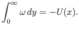 |
(8.58) |
Furthermore, from Equations (8.40), (8.47), and (8.52), the
-component of the viscous force per unit area acting on the surface of
the obstacle is
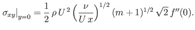 |
(8.59) |
It is convenient to parameterize this quantity in terms of a skin friction coefficient,
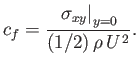 |
(8.60) |
It follows that
![$\displaystyle c_f(x) = \frac{(m+1)^{1/2}\,\sqrt{2}\,f''(0)}{[{\rm Re}(x)]^{1/2}},$](img2948.png) |
(8.61) |
where
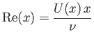 |
(8.62) |
is the effective Reynolds number of the flow on the outer edge of the layer at position
. Hence,
 .
Finally, according to Equation (8.41), the width of the boundary layer is approximately
.
Finally, according to Equation (8.41), the width of the boundary layer is approximately
![$\displaystyle \frac{\delta(x)}{x} \simeq \frac{1}{[{\rm Re}(x)]^{\,1/2}},$](img2951.png) |
(8.63) |
which implies that
 .
.
Figure:
 calculated as a function of
  for solutions of the Falkner-Skan equation.
 |
If  then the external tangential velocity profile,
, corresponds to that of irrotational inviscid
flow incident, in a symmetric fashion, on a semi-infinite wedge whose apex subtends an angle
then the external tangential velocity profile,
, corresponds to that of irrotational inviscid
flow incident, in a symmetric fashion, on a semi-infinite wedge whose apex subtends an angle
 , where
 . (See Section 5.10, and Figure 5.10.) In this case,
  can be interpreted as the tangential velocity a distance
along the surface of the wedge from its apex (in the direction of the flow).
By analogy, if
can be interpreted as the tangential velocity a distance
along the surface of the wedge from its apex (in the direction of the flow).
By analogy, if  then the external velocity profile corresponds to that of irrotational inviscid flow parallel to a semi-infinite flat
plate (which can be thought of as a wedge whose apex subtends zero angle). In this case,
can be interpreted as the tangential velocity
a distance
along the surface of the plate from its leading edge (in the direction of the flow). (See Section 8.5.)
Finally, if
then the external velocity profile corresponds to that of irrotational inviscid flow parallel to a semi-infinite flat
plate (which can be thought of as a wedge whose apex subtends zero angle). In this case,
can be interpreted as the tangential velocity
a distance
along the surface of the plate from its leading edge (in the direction of the flow). (See Section 8.5.)
Finally, if  then the
external velocity profile is that of symmetric irrotational inviscid flow over the back surface of a semi-infinite wedge whose apex
subtends an angle
then the
external velocity profile is that of symmetric irrotational inviscid flow over the back surface of a semi-infinite wedge whose apex
subtends an angle
 , where
 . (See Section 5.11, and Figure 5.11.)
In this case,
can be interpreted as the tangential velocity a distance
along the surface of the wedge from its apex (in the
direction of the flow).
. (See Section 5.11, and Figure 5.11.)
In this case,
can be interpreted as the tangential velocity a distance
along the surface of the wedge from its apex (in the
direction of the flow).
Unfortunately, the Falkner-Skan equation, (8.53), possesses no general analytic solutions. However, this equation is relatively straightforward to solve via numerical methods.
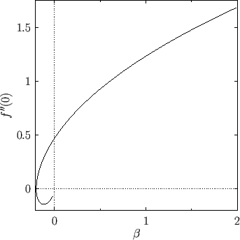
Figure 8.2 shows
, calculated numerically as a function of
 , for the solutions of Equation (8.53) that
satisfy the boundary conditions (8.55)-(8.57). In addition, Figure 8.3 shows
, for the solutions of Equation (8.53) that
satisfy the boundary conditions (8.55)-(8.57). In addition, Figure 8.3 shows  versus
, calculated numerically
for various different values of
.
Because
versus
, calculated numerically
for various different values of
.
Because
 as
as
 , solutions of the Falkner-Skan equation with
 have no physical significance. For
  , it can be seen, from Figures 8.2 and 8.3, that there is a single
solution branch characterized by
, it can be seen, from Figures 8.2 and 8.3, that there is a single
solution branch characterized by
 and
and  . This branch is termed the forward flow branch, because it
is such that the tangential velocity,
. This branch is termed the forward flow branch, because it
is such that the tangential velocity,
 , is in the same direction as the
external tangential velocity [i.e.,
, is in the same direction as the
external tangential velocity [i.e.,
 ] across the whole layer (i.e.,
 ).
The forward flow branch is characterized by a positive skin friction coefficient,
).
The forward flow branch is characterized by a positive skin friction coefficient,
 .
It can also be seen that for
.
It can also be seen that for  there exists a second solution branch, which is termed the reversed flow
branch, because it is such that the tangential velocity is in the opposite direction to the
external tangential velocity in the region of the layer immediately adjacent to the surface of the obstacle (which corresponds to
there exists a second solution branch, which is termed the reversed flow
branch, because it is such that the tangential velocity is in the opposite direction to the
external tangential velocity in the region of the layer immediately adjacent to the surface of the obstacle (which corresponds to  ).
The reversed flow branch is characterized by a negative skin friction coefficient. The reversed flow
solutions are probably unphysical, because reversed flow close to the wall is generally associated
with a phenomenon known as boundary layer
separation (see Section 8.10) that invalidates the boundary layer orderings.
It can be seen that the two
solution branches merge together at
).
The reversed flow branch is characterized by a negative skin friction coefficient. The reversed flow
solutions are probably unphysical, because reversed flow close to the wall is generally associated
with a phenomenon known as boundary layer
separation (see Section 8.10) that invalidates the boundary layer orderings.
It can be seen that the two
solution branches merge together at
 ,
which corresponds to
,
which corresponds to
 . Moreover, there are no solutions to the Falkner-Skan equation with
 or
or  .
The disappearance of solutions when
becomes too negative (i.e., when the deceleration of the
external flow becomes too large) is also related to boundary layer separation.
.
The disappearance of solutions when
becomes too negative (i.e., when the deceleration of the
external flow becomes too large) is also related to boundary layer separation.
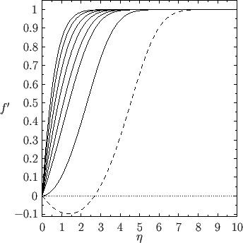
Figure:
Solutions of the Falkner-Skan equation. In order from the left to the right, the various solid curves correspond to forward flow solutions calculated with  ,
,  ,
,  ,
,  , 0
,
, 0
,
 , and
, and  , respectively. The dashed curve shows a reversed flow solution calculated with
  .
.
 |
Next: Boundary Layer on a
Up: Incompressible Boundary Layers
Previous: Boundary Layer Equations
Richard Fitzpatrick
2016-03-31
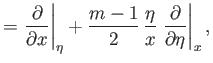
![$\displaystyle =\left[\frac{(m+1)\,U_0\,x^{\,m-1}}{2\,\nu}\right]^{1/2}\left.\frac{\partial}{\partial\eta}\right\vert _x.$](img2926.png)