Next: Self-Similar Boundary Layers
Up: Incompressible Boundary Layers
Previous: No Slip Condition
Boundary Layer Equations
Consider a rigid stationary obstacle whose surface is (locally) flat, and corresponds to the  -
- plane. Let this
surface be in contact with a high Reynolds
number fluid that occupies the region
plane. Let this
surface be in contact with a high Reynolds
number fluid that occupies the region  . (See Figure 8.1.) Let
  be the typical normal thickness of the boundary layer.
The layer thus extends over the region
be the typical normal thickness of the boundary layer.
The layer thus extends over the region
 . The fluid that occupies the region
 ,
and thus lies outside
the layer, is assumed to be both irrotational and (effectively) inviscid. On the other hand, viscosity must be included in the
equation of motion of the fluid within the layer. The fluid both inside and outside the layer is assumed to
be incompressible.
,
and thus lies outside
the layer, is assumed to be both irrotational and (effectively) inviscid. On the other hand, viscosity must be included in the
equation of motion of the fluid within the layer. The fluid both inside and outside the layer is assumed to
be incompressible.
Figure 8.1:
A boundary layer.
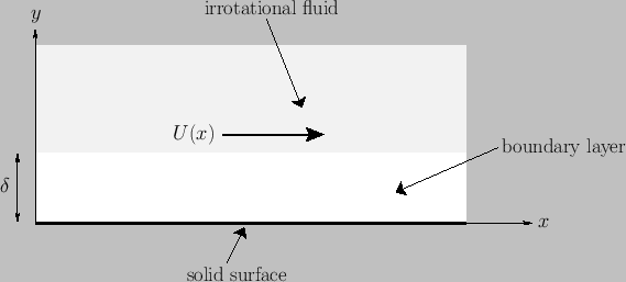 |
Suppose that the equations of irrotational flow have already been solved to determine the fluid velocity outside the boundary
layer. This velocity must be such that its normal component is zero at the outer edge of the layer (i.e., at
 ). On the other hand, the tangential component of the fluid velocity at the outer edge of the layer,
  (say), is generally non-zero.
Here, we are assuming, for the sake of simplicity, that there is no spatial variation in the
-direction, so
that both the irrotational flow and the boundary layer are effectively two-dimensional.
Likewise, we are also assuming that all flows are steady, so that any time variation can be neglected.
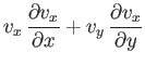
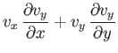
The motion of the fluid within the boundary layer is governed by the equations of steady-state, incompressible,
two-dimensional, viscous flow, which take the form (see Section 1.14)
(say), is generally non-zero.
Here, we are assuming, for the sake of simplicity, that there is no spatial variation in the
-direction, so
that both the irrotational flow and the boundary layer are effectively two-dimensional.
Likewise, we are also assuming that all flows are steady, so that any time variation can be neglected.
The motion of the fluid within the boundary layer is governed by the equations of steady-state, incompressible,
two-dimensional, viscous flow, which take the form (see Section 1.14)
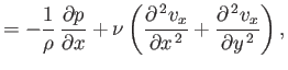
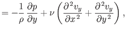
where  is the (constant) density, and
  the kinematic viscosity. Here, Equation (8.1) is the
equation of continuity, whereas Equations (8.2) and (8.3) are the
- and
the kinematic viscosity. Here, Equation (8.1) is the
equation of continuity, whereas Equations (8.2) and (8.3) are the
- and  -components of the fluid equation of motion,
respectively. The boundary conditions at the outer edge of the layer, where it interfaces with the irrotational
fluid, are
-components of the fluid equation of motion,
respectively. The boundary conditions at the outer edge of the layer, where it interfaces with the irrotational
fluid, are
as
 . Here,
  is the fluid pressure at the outer edge of the layer, and
 |
(8.6) |
(because  , and viscosity is negligible, just outside the layer).
The boundary conditions at the inner edge of the layer, where it interfaces with the impenetrable surface, are
, and viscosity is negligible, just outside the layer).
The boundary conditions at the inner edge of the layer, where it interfaces with the impenetrable surface, are
Of course, the first of these constraints corresponds to the no slip condition.
Let  be a typical value of the external tangential velocity,
, and let
be a typical value of the external tangential velocity,
, and let  be the typical variation length-scale
of this quantity. It is reasonable to suppose that
and
are also the characteristic tangential flow velocity and variation length-scale in the
-direction, respectively, of the boundary layer.
Of course,
is the typical variation length-scale of the layer in the
-direction. Moreover,
be the typical variation length-scale
of this quantity. It is reasonable to suppose that
and
are also the characteristic tangential flow velocity and variation length-scale in the
-direction, respectively, of the boundary layer.
Of course,
is the typical variation length-scale of the layer in the
-direction. Moreover,
 ,
because the layer is assumed to be thin.
It is helpful to define the normalized variables
,
because the layer is assumed to be thin.
It is helpful to define the normalized variables
 |
 |
(8.9) |
 |
 |
(8.10) |
 |
 |
(8.11) |
 |
 |
(8.12) |
 |
 |
(8.13) |
where  and
and  are constants.
All of these variables are designed to be
are constants.
All of these variables are designed to be
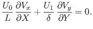
 inside the layer. Equation (8.1) yields
 |
(8.14) |
In order for the terms in this equation to balance one another, we need
 |
(8.15) |
In other words, within the layer, continuity requires the typical flow velocity in the
-direction,
, to be much smaller than
that in the
-direction,
.
Equation (8.2) gives
![$\displaystyle \frac{U_0^{\,2}}{L}\left(V_x\,\frac{\partial V_x}{\partial X} + V...
...\,2} V_x}{\partial X^{\,2}}+\frac{\partial^{\,2} V_x}{\partial Y^{\,2}}\right].$](img2889.png) |
(8.16) |
In order for the pressure term on the right-hand side of the previous equation to be of similar magnitude to the advective terms on the
left-hand side, we require that
 |
(8.17) |
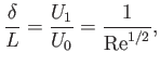
Furthermore, in order for the viscous term on the right-hand side to balance the other terms, we
need
 |
(8.18) |
where
 |
(8.19) |
is the Reynolds number of the flow external to the layer. (See Section 1.16.) The
assumption that
can be seen to imply that
 . In other words, the normal thickness of the boundary layer separating an irrotational flow pattern
from a rigid surface is only much less than the typical variation length-scale of the pattern when the Reynolds
number of the flow is much greater than unity.
. In other words, the normal thickness of the boundary layer separating an irrotational flow pattern
from a rigid surface is only much less than the typical variation length-scale of the pattern when the Reynolds
number of the flow is much greater than unity.
Equation (8.3) yields
![$\displaystyle \frac{1}{{\rm Re}}\left(V_x\,\frac{\partial V_y}{\partial X} + V_...
...\,2} V_y}{\partial X^{\,2}}+\frac{\partial^{\,2} V_y}{\partial Y^{\,2}}\right].$](img2893.png) |
(8.20) |
In the limit
, this reduces to
 |
(8.21) |
Hence,
 , where
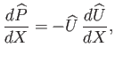 |
(8.22) |
 , and use has been made of Equation (8.6). In other words, the pressure
is uniform across the layer, in the direction normal to the surface of the obstacle, and is thus the same as that on the
outer edge of the layer.
, and use has been made of Equation (8.6). In other words, the pressure
is uniform across the layer, in the direction normal to the surface of the obstacle, and is thus the same as that on the
outer edge of the layer.
Retaining only
terms, our final set of normalized layer equations becomes
subject to the boundary conditions
 |
(8.25) |
and
In unnormalized form, the previous set of layer equations are written
subject to the boundary conditions
 |
(8.30) |
(note that  really means
), and
really means
), and
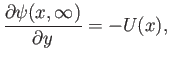
Equation (8.28) can be automatically satisfied by expressing the flow velocity in terms of a
stream function: that is,
In this case, Equation (8.29) reduces to
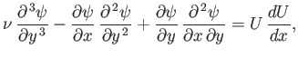 |
(8.35) |
subject to the boundary conditions
 |
(8.36) |
and
To lowest order, the vorticity internal to the layer,

 , is given by
 |
(8.39) |
whereas the
-component of the viscous force per unit area acting on the surface of the obstacle is written (see Section 1.18)
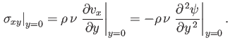 |
(8.40) |
Next: Self-Similar Boundary Layers
Up: Incompressible Boundary Layers
Previous: No Slip Condition
Richard Fitzpatrick
2016-03-31