Next: 2-d problem with Neumann
Up: The diffusion equation
Previous: An improved 1-d solution
Let us consider the solution of the diffusion equation in two dimensions. Suppose
that
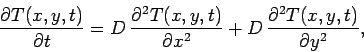 |
(214) |
for
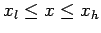 , and
, and  . Suppose that
  satisfies mixed
boundary conditions in the
satisfies mixed
boundary conditions in the  -direction:
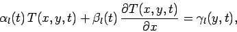 |
(215) |
at  , and
, and
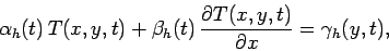 |
(216) |
at  . Here,
  ,
,  , etc., are known functions of
  ,
whereas
,
whereas  ,
,  are known functions of
  and .
Furthermore, suppose that satisfies the following simple Dirichlet boundary
conditions in the -direction:
and .
Furthermore, suppose that satisfies the following simple Dirichlet boundary
conditions in the -direction:
 |
(217) |
As before, we discretize in time on the uniform grid
 , for
, for
 .
Furthermore, in the -direction, we discretize on the uniform grid
.
Furthermore, in the -direction, we discretize on the uniform grid
 , for
, for
 , where
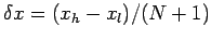 . Finally, in the -direction, we discretize
on the uniform grid
. Finally, in the -direction, we discretize
on the uniform grid
 , for
, for  , where
 .
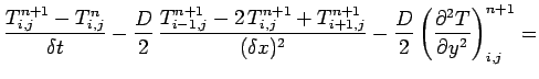
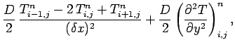
Adopting the Crank-Nicholson temporal differencing scheme discussed in Sect. 6.6, and
the second-order spatial differencing scheme outlined in
Sect. 5.2, Eq. (214) yields
.
Adopting the Crank-Nicholson temporal differencing scheme discussed in Sect. 6.6, and
the second-order spatial differencing scheme outlined in
Sect. 5.2, Eq. (214) yields
 |
|
|
|
 |
|
|
(218) |
where
 . The discretized boundary conditions
take the form
. The discretized boundary conditions
take the form
plus
 |
(221) |
Here,
 , etc., and
 , etc.
Adopting the Fourier method introduced in Sect. 5.7, we
write the  in terms of their Fourier-sine harmonics:
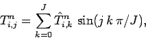 |
(222) |
which automatically satisfies the boundary conditions (221).
The above expression can be inverted to give (see Sect. 5.9)
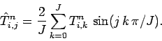 |
(223) |
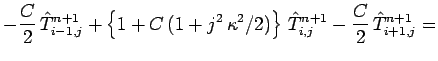
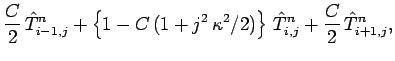
When Eq. (218) is written in terms of the
 , it reduces to
 |
|
|
|
 |
|
|
(224) |
for  , and . Here,
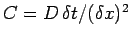 , and
, and
 .
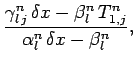
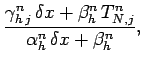
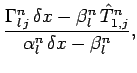
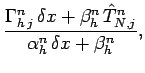
Moreover, the boundary conditions (219) and (220) yield
.
Moreover, the boundary conditions (219) and (220) yield
where
 |
(227) |
etc. Equations (224)--(226) constitute a set of  uncoupled tridiagonal matrix equations for the
 , with one
equation for each separate value of
, with one
equation for each separate value of  .
.
In order to advance our solution by one time-step, we first Fourier transform the
and the boundary conditions, according to Eqs. (223) and (227).
Next, we invert the tridiagonal equations (224)--(226) to
obtain the
. Finally, we reconstruct the via
Eq. (222).
Next: 2-d problem with Neumann
Up: The diffusion equation
Previous: An improved 1-d solution
Richard Fitzpatrick
2006-03-29