


Next: An example tridiagonal matrix
Up: Poisson's equation
Previous: Introduction
1-d problem with Dirichlet boundary conditions
As a simple test case, let us consider the solution of Poisson's equation
in one dimension. Suppose that
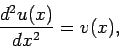 |
(113) |
for
 , subject to the Dirichlet boundary conditions
 and
and  .
.
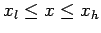
As a first step, we divide the domain
into equal
segments whose vertices are located at the grid-points
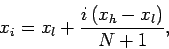 |
(114) |
for  . The boundaries,
  and
and  , correspond to
  and
and  ,
respectively.
,
respectively.
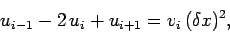
Next, we discretize the differential term  on the grid-points. The most
straightforward discretization is
on the grid-points. The most
straightforward discretization is
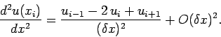 |
(115) |
Here,
 , and
, and
 . This type
of discretization is termed a second-order, central difference scheme.
It is
``second-order'' because the truncation error is
. This type
of discretization is termed a second-order, central difference scheme.
It is
``second-order'' because the truncation error is  , as can
easily be demonstrated via Taylor expansion. Of course, an
, as can
easily be demonstrated via Taylor expansion. Of course, an  th order scheme
would have a truncation error which is
th order scheme
would have a truncation error which is  .
It is a ``central difference'' scheme because it is symmetric about the central
grid-point,
.
It is a ``central difference'' scheme because it is symmetric about the central
grid-point,  .
Our discretized version of Poisson's equation takes the form
.
Our discretized version of Poisson's equation takes the form
 |
(116) |
for , where
 . Furthermore,
  and
and  .
.
It is helpful to regard the above set of discretized equations as a matrix equation.
Let
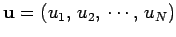 be the vector of the
  -values,
and let
-values,
and let
![\begin{displaymath}
{\bf w} = [v_1\,(\delta x)^2 - u_l,\, v_2\,(\delta x)^2,\, v...
...\,\cdots,\, v_{N-1}\, (\delta x)^2,\,
v_N\,(\delta x)^2 - u_h]
\end{displaymath}](img659.png) |
(117) |
be the vector of the source terms. The discretized equations can be written
as:
 |
(118) |
The matrix  takes the form
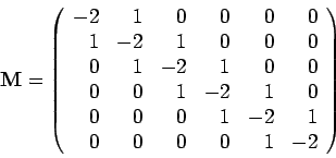 |
(119) |
for  . The generalization to other
  values is fairly obvious.
Matrix is termed a tridiagonal matrix, since only those elements which lie on
the three leading diagonals are non-zero.
values is fairly obvious.
Matrix is termed a tridiagonal matrix, since only those elements which lie on
the three leading diagonals are non-zero.
The formal solution to Eq. (118) is
 |
(120) |
where  is the inverse matrix to . Unfortunately, the most efficient
general purpose algorithm for inverting an
is the inverse matrix to . Unfortunately, the most efficient
general purpose algorithm for inverting an  matrix--namely, Gauss-Jordan elimination
with partial pivoting--requires
matrix--namely, Gauss-Jordan elimination
with partial pivoting--requires  arithmetic operations. It is fairly clear that this
is a disastrous scaling for finite-difference solutions of Poisson's equation.
Every time we doubled the resolution (i.e., doubled the number of grid-points) the
required cpu time would increase by a factor of about eight. Consequently, adding a second dimension (which
effectively requires the number of grid-points to be squared) would be prohibitively expensive
in terms of cpu time. Fortunately, there is a well-known trick for inverting an
tridiagonal
matrix which only requires
arithmetic operations. It is fairly clear that this
is a disastrous scaling for finite-difference solutions of Poisson's equation.
Every time we doubled the resolution (i.e., doubled the number of grid-points) the
required cpu time would increase by a factor of about eight. Consequently, adding a second dimension (which
effectively requires the number of grid-points to be squared) would be prohibitively expensive
in terms of cpu time. Fortunately, there is a well-known trick for inverting an
tridiagonal
matrix which only requires  arithmetic operations.
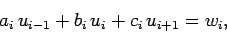
Consider a general tridiagonal matrix equation
 .
Let
.
Let  ,
,  , and
, and  be the vectors of the left, center and right
diagonal elements of the matrix, respectively
Note that
be the vectors of the left, center and right
diagonal elements of the matrix, respectively
Note that  and
and  are undefined, and can be conveniently
set to zero. Our matrix equation can now be written
are undefined, and can be conveniently
set to zero. Our matrix equation can now be written
 |
(121) |
for .
Let us search for a solution of the form
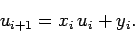 |
(122) |
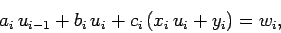
Substitution into Eq. (121) yields
 |
(123) |
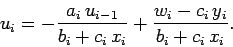
which can be rearranged to give
 |
(124) |
However, if Eq. (122) is general then we can write
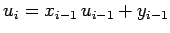 .
Comparison with the previous equation yields
.
Comparison with the previous equation yields
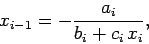 |
(125) |
and
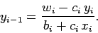 |
(126) |
We can now solve our tridiagonal matrix equation in two stages. In the first stage, we scan
up the leading diagonal from  to
to  using Eqs. (125) and (126). Thus,
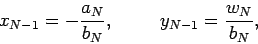 |
(127) |
since  . Furthermore,
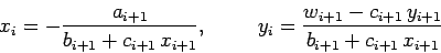 |
(128) |
for 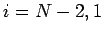 . Finally,
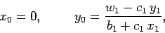 |
(129) |
since  . We have now defined all of the and
  . In the second stage,
we scan down the leading diagonal from to
. In the second stage,
we scan down the leading diagonal from to  using Eq. (122).
Thus,
using Eq. (122).
Thus,
 |
(130) |
since  , and
, and
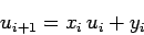 |
(131) |
for  . We have now inverted our tridiagonal matrix equation using arithmetic
operations.
. We have now inverted our tridiagonal matrix equation using arithmetic
operations.
Clearly, we can use the above algorithm to invert Eq. (118), with the source terms
specified in Eq. (117), and the diagonals of matrix given by
 for
for  , plus
  for , and
  for .
for .
Next: An example tridiagonal matrix
Up: Poisson's equation
Previous: Introduction
Richard Fitzpatrick
2006-03-29