An improved 1-d solution of the diffusion equation

Let us now solve the simple diffusion problem introduced in Sect. 6.4 with the above listed Crank-Nicholson routine. Figure 73 shows a comparison between the analytic and numerical solutions for a calculation performed using $D=1$, $x_0=5$, $t_0=0.1$, $\delta t = 0.1$, and $N=100$. It can be seen that the analytic and numerical solutions are in excellent agreement. Note, however, that the time-step used in this calculation (i.e., $\delta t = 0.1$) is much larger than that used in our previous calculation (i.e., $\delta t = 4\times 10^{-3}$), which employed an explicit differencing scheme--see Fig. 71. According to Eq. (209), an explicit scheme is limited to time-steps less than about $5\times 10^{-3}$ for the problem under investigation. Thus, we have been able to exceed this limit by a factor of 20 with our implicit scheme, yet still maintain numerical stability. Note that our Crank-Nicholson scheme is able to obtain accurate results with a time-step as large as $0.1$ because it is second-order in time.

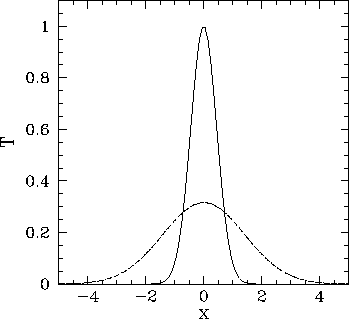
Figure 73: Diffusive evolution of a 1-d Gaussian pulse. Numerical calculation performed using $D=1$, $x_0=5$, $\delta t = 0.1$, and $N=100$. The pulse is evolved from $t=0.1$ to $t=1$. The solid curve shows the initial condition at $t=0.1$, the dashed curve the numerical solution at $t=1$, and the dotted curve (obscured by the dashed curve) the analytic solution at $t=1$.