An example 1-d solution of the diffusion equation

Let us now solve the diffusion equation in 1-d using the finite difference technique discussed above. We seek the solution of Eq. (191) in the region $-x_0 \leq x \leq x_0$, subject to the initial condition

$$T(x,t_0) = \exp\!\left(\frac{-x^2}{4\,D\,t_0}\right),$$ (200)

where $t_0>0$. The spatial boundary conditions are

$$T(\pm x_0,t) = \sqrt{\frac{t_0}{t}}\, \exp\!\left(\frac{-x_0^2}{4\,D\,t}\right).$$ (201)

Of course, we can solve this problem analytically to give

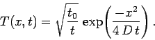$$T(x,t) =\sqrt{\frac{t_0}{t}}\, \exp\!\left(\frac{-x^2}{4\,D\,t}\right).$$ (202)

Note that the above equation describes a Gaussian pulse which gradually decreases in height and broadens in width in such a manner that its area is conserved. The width of the pulse varies approximately as

$${\mit\Delta}x \sim \sqrt{D\,t}.$$ (203)

Moreover, the pulse approaches a $\delta$-function as $t\rightarrow 0$.

Figure 71: Diffusive evolution of a 1-d Gaussian pulse. Numerical calculation performed using $D=1$, $x_0=5$, $\delta t = 4\times 10^{-3}$, and $N=100$. The pulse is evolved from $t=0.1$ to $t=1$. The solid curve shows the initial condition at $t=0.1$, the dashed curve the numerical solution at $t=1$, and the dotted curve (obscured by the dashed curve) the analytic solution at $t=1$.

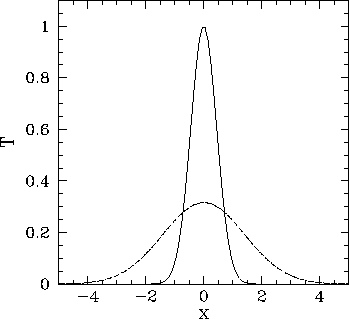Figure 71 shows a comparison between the analytic and numerical solutions for a calculation performed using $D=1$, $x_0=5$, $t_0=0.1$, $\delta t = 4\times 10^{-3}$, and $N=100$. It can be seen that the analytic and numerical solutions are in excellent agreement.

Figure 72: Diffusive evolution of a 1-d Gaussian pulse. Numerical calculation performed using $D=1$, $x_0=5$, $\delta t = 4\times 10^{-3}$, and $N=125$. The simulation is started at $t=0.1$. The top-left, top-right, bottom-left, and bottom-right panels show the solution at $t=0.45$, $t=0.46$, $t=0.47$, and $t=0.48$, respectively.

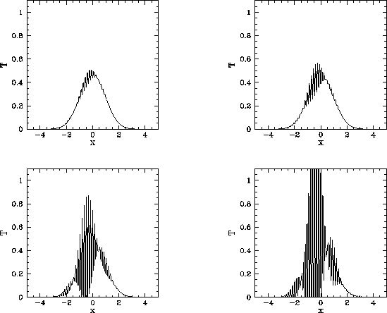It is reasonable to expect that as $N$ increases at fixed $\delta t$ (i.e., the spatial resolution increases at fixed temporal resolution) the numerical solution should become more and more accurate. This is indeed the case--at least, until $N$ exceeds a critical value. Beyond this value, there is a catastrophic breakdown in the numerical solution. This breakdown is illustrated in Fig. 72. It can be seen that the solution develops rapidly growing short-wavelength oscillations. Indeed, the solution eventually becomes effectively infinite. Let us investigate this unusual and rather disturbing phenomenon.