Next: An example 1-d diffusion
Up: The diffusion equation
Previous: Introduction
Consider the solution of the diffusion equation in one dimension.
Suppose that
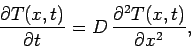 |
(191) |
for
 , subject to the mixed spatial boundary conditions
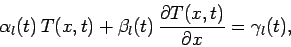 |
(192) |
at  , and
, and
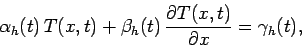 |
(193) |
at  . Here,
  ,
,  , etc., are known functions of time.
Of course,
, etc., are known functions of time.
Of course,  must be specified at some initial time
  .
.
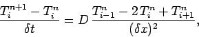
Equation (191) needs to be discretized in both time and space.
In time, we discretize
on the equally spaced grid
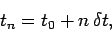 |
(194) |
where  is the time-step. Adopting a
simple first-order differencing scheme, Eq. (191) becomes
is the time-step. Adopting a
simple first-order differencing scheme, Eq. (191) becomes
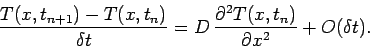 |
(195) |
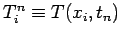
In space,
we discretize on the usual equally spaced grid-points specified in Eq. (114),
and approximate  via the second-order, central difference scheme
introduced in Eq. (115). The spatial boundary conditions are discretized in a similar
manner to Eqs. (134) and (135). Thus, Eq. (195) yields
via the second-order, central difference scheme
introduced in Eq. (115). The spatial boundary conditions are discretized in a similar
manner to Eqs. (134) and (135). Thus, Eq. (195) yields
 |
(196) |
or
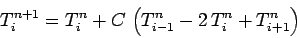 |
(197) |
for  , where
 , and
, and
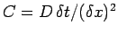 .
The discretized boundary conditions take the form
.
The discretized boundary conditions take the form
where
 , etc. The discretization scheme outlined above
is termed first-order in time and second-order in space.
, etc. The discretization scheme outlined above
is termed first-order in time and second-order in space.
Equations (197)-(199) constitute a fairly straightforward iterative scheme which
can be used to evolve the  in time.
Next: An example 1-d diffusion
Up: The diffusion equation
Previous: Introduction
Richard Fitzpatrick
2006-03-29