


Next: 1-d problem with mixed
Up: The diffusion equation
Previous: The diffusion equation
The diffusion equation
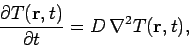 |
(187) |
where  is the (uniform) coefficient of diffusion, describes many interesting physical
phenomena. For instance, in heat conduction we can write
is the (uniform) coefficient of diffusion, describes many interesting physical
phenomena. For instance, in heat conduction we can write
 |
(188) |
where  is the heat flux,
  the temperature, and
  the coefficient
of thermal conductivity. The above equation merely states that heat flows down a temperature
gradient. In the absence of sinks or sources of heat, energy conservation
requires that
the coefficient
of thermal conductivity. The above equation merely states that heat flows down a temperature
gradient. In the absence of sinks or sources of heat, energy conservation
requires that
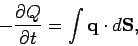 |
(189) |
where  is the thermal energy contained in some volume
  bounded by a closed surface
  .
The above equation states that the rate of decrease of the thermal energy content of
volume
equals the instantaneous heat flux flowing across its boundary.
However,
.
The above equation states that the rate of decrease of the thermal energy content of
volume
equals the instantaneous heat flux flowing across its boundary.
However,
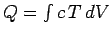 , where
  is the heat capacity per unit volume. Making
use of the previous
equations, as well as the divergence theorem, we obtain the following diffusion
equation for the temperature:
is the heat capacity per unit volume. Making
use of the previous
equations, as well as the divergence theorem, we obtain the following diffusion
equation for the temperature:
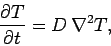 |
(190) |
where  . In a typical heat conduction problem, we are given the
temperature
. In a typical heat conduction problem, we are given the
temperature
 at some initial time
  , and then asked
to evaluate
, and then asked
to evaluate  at all subsequent times. Such a problem is
known as an initial value problem. The spatial boundary conditions can be either
of type Dirichlet (i.e., specified on the boundary), type
Neumann (i.e.,
at all subsequent times. Such a problem is
known as an initial value problem. The spatial boundary conditions can be either
of type Dirichlet (i.e., specified on the boundary), type
Neumann (i.e.,  specified on the boundary), or some combination.
Next: 1-d problem with mixed
Up: The diffusion equation
Previous: The diffusion equation
Richard Fitzpatrick
2006-03-29