Next: 2-d problem with Neumann
Up: Poisson's equation
Previous: An example solution of
2-d problem with Dirichlet boundary conditions
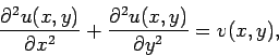
Let us consider the solution of Poisson's equation
in two dimensions. Suppose that
 |
(146) |
for
 , and
, and
 . By direct analogy
with our previous method of solution in the 1-d case, we could discretize
the above 2-d problem using a second-order, central difference scheme in both
the
. By direct analogy
with our previous method of solution in the 1-d case, we could discretize
the above 2-d problem using a second-order, central difference scheme in both
the  - and
- and  -directions. Unfortunately, such a discretization scheme yields a
set of equations which cannot be reduced to a simple tridiagonal matrix equation.
In fact, all of the efficient numerical algorithms for solving this type of problem are
iterative in nature. For instance, the Jacobi method, the
Gauss-Seidel method, the successive over-relaxation method, and the multi-grid
method.34Regrettably, unless such iteration methods are extremely sophisticated (e.g., the multi-grid method),
and, hence,
beyond the scope of this course,
they tend to converge very poorly. In the following,
rather than discuss iterative methods which do not work
very well, we shall instead discuss a non-iterative method which works effectively
for a restricted set of problems. The method in question is termed a spectral method, since
it involves expanding
-directions. Unfortunately, such a discretization scheme yields a
set of equations which cannot be reduced to a simple tridiagonal matrix equation.
In fact, all of the efficient numerical algorithms for solving this type of problem are
iterative in nature. For instance, the Jacobi method, the
Gauss-Seidel method, the successive over-relaxation method, and the multi-grid
method.34Regrettably, unless such iteration methods are extremely sophisticated (e.g., the multi-grid method),
and, hence,
beyond the scope of this course,
they tend to converge very poorly. In the following,
rather than discuss iterative methods which do not work
very well, we shall instead discuss a non-iterative method which works effectively
for a restricted set of problems. The method in question is termed a spectral method, since
it involves expanding  and
and  as truncated Fourier series in the -direction.
Suppose that  satisfies mixed boundary conditions in the -direction: i.e.,
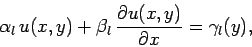 |
(147) |
at  , and
, and
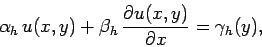 |
(148) |
at  . Here,
  ,
,  , etc., are known constants,
whereas
, etc., are known constants,
whereas  ,
,  are known functions of .
Furthermore, suppose that satisfies the following simple Dirichlet boundary
conditions in the -direction:
are known functions of .
Furthermore, suppose that satisfies the following simple Dirichlet boundary
conditions in the -direction:
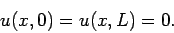 |
(149) |
Note that, since is a potential, and, hence, probably undetermined to an
arbitrary additive constant, the above boundary conditions are equivalent to
demanding that take the
same constant value on both the upper and lower boundaries in the -direction.
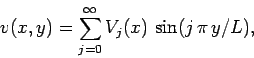
Let us write as a Fourier series in the -direction:
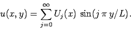 |
(150) |
Note that the above expression for automatically satisfies the boundary conditions
in the -direction. The
 functions are orthogonal, and form a complete set, in
the interval
functions are orthogonal, and form a complete set, in
the interval  . In fact,
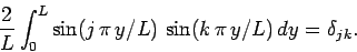 |
(151) |
Thus, we can write the source term as
 |
(152) |
where
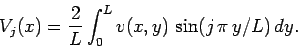 |
(153) |
Furthermore, the boundary conditions in the -direction become
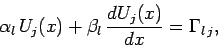 |
(154) |
at , and
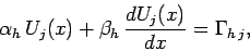 |
(155) |
at , where
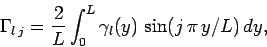 |
(156) |
etc.
Substituting Eqs. (150) and (152) into Eq. (146), and equating
the coefficients of the
(since these functions are orthogonal), we
obtain
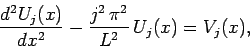 |
(157) |
for  . Now, we can discretize the problem in the -direction by truncating our
Fourier expansion: i.e., by only solving the above equations for
. Now, we can discretize the problem in the -direction by truncating our
Fourier expansion: i.e., by only solving the above equations for  , rather
than . This is essentially equivalent to discretization in the -direction on the
equally-spaced grid-points
, rather
than . This is essentially equivalent to discretization in the -direction on the
equally-spaced grid-points
 .
The problem is discretized in the -direction by dividing the domain
into equal segments, according to Eq. (114), and approximating
.
The problem is discretized in the -direction by dividing the domain
into equal segments, according to Eq. (114), and approximating  via the
second-order, central difference scheme specified in Eq. (115). Thus, we obtain
via the
second-order, central difference scheme specified in Eq. (115). Thus, we obtain
 |
(158) |
for  and . Here,
 ,
,
 , and
, and
 . The
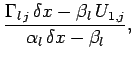
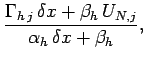
boundary conditions (154) and (155) discretize to give:
. The
boundary conditions (154) and (155) discretize to give:
for . Eqs. (158), (159), and (160) constitute a set of  uncoupled tridiagonal matrix equations (with one equation for each separate
  value).
These equations can be inverted, using the algorithm discussed in Sect. 5.4, to
give the
value).
These equations can be inverted, using the algorithm discussed in Sect. 5.4, to
give the  . Finally, the
  values can be reconstructed from Eq. (150).
Hence, we have solved the problem.
values can be reconstructed from Eq. (150).
Hence, we have solved the problem.
Next: 2-d problem with Neumann
Up: Poisson's equation
Previous: An example solution of
Richard Fitzpatrick
2006-03-29