Up to now, we have only discussed wave mechanics for a particle moving in one dimension. However, the
generalization to a particle moving in three dimensions is fairly straightforward.
A massive particle moving in three dimensions
has a complex wavefunction of the form [cf., Equation (11.15)]
 |
(11.151) |
where  is a complex constant, and
 . Here, the wavevector,
  , and
the angular frequency,
, and
the angular frequency,  , are related to the particle momentum,
  , and energy,
  , according
to [cf., Equation (11.3)]
, according
to [cf., Equation (11.3)]
 |
(11.152) |
and [cf., Equation (11.1)]
 |
(11.153) |
respectively. Generalizing the
analysis of Section 11.5, the three-dimensional version of Schrödinger's
equation is [cf., Equation (11.23)]
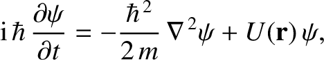 |
(11.154) |
where the differential operator
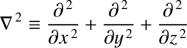 |
(11.155) |
is known as the Laplacian. The interpretation of a three-dimensional wavefunction is that the
probability of simultaneously finding the particle between  and
and  , between
  and
and  , and
between
, and
between  and
and  , at time
  is [cf., Equation (11.26)]
 |
(11.156) |
Moreover, the normalization condition for the wavefunction becomes [cf., Equation (11.28)]
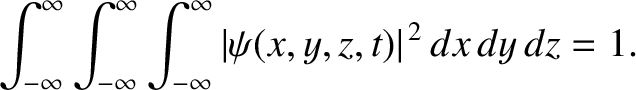 |
(11.157) |
It can be demonstrated that Schrödinger's equation, (11.154), preserves the normalization
condition, (11.157), of a localized wavefunction (Gasiorowicz 1996).
Heisenberg's uncertainty principle generalizes to [cf., Equation (11.56)]
 |
 |
(11.158) |
 |
|
(11.159) |
 |
 |
(11.160) |
 |
(11.161) |
where the stationary wavefunction,
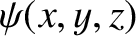 , satisfies [cf., Equation (11.62)]
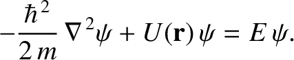 |
(11.162) |