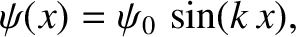
Consider separable solutions to Schrödinger's equation of the form
 |
(11.59) |
According to Equation (11.20), such solutions have definite energies
 . For this reason,
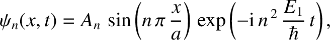
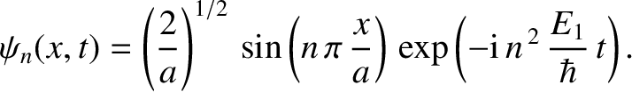
they are usually written
. For this reason,
they are usually written
 |
(11.60) |
The probability of finding the particle between  and
and 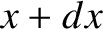 at time
  is
is
 |
(11.61) |
This probability is time independent. For this reason, states whose wavefunctions are of the
form (11.60) are known as stationary states. Moreover,  is called a stationary
wavefunction. Substituting (11.60) into Schrödinger's equation, (11.23), we
obtain the following differential equation for ;
is called a stationary
wavefunction. Substituting (11.60) into Schrödinger's equation, (11.23), we
obtain the following differential equation for ;
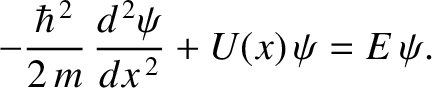 |
(11.62) |
This equation is called the time-independent Schrödinger equation.
Consider a particle trapped in a one-dimensional square potential well, of infinite depth, which is such that
![\begin{displaymath}U(x) = \left\{
\begin{array}{lll}
0&\mbox{\hspace{0.5cm}}&0\l...
... \leq a\\ [0.5ex]
\infty &&\mbox{otherwise}
\end{array}\right..\end{displaymath}](img3921.png) |
(11.63) |
The particle is excluded from the region  or
or  , so
, so  in this region (i.e., there
is zero probability of finding the particle outside the well). Within the well, a particle
of definite energy
in this region (i.e., there
is zero probability of finding the particle outside the well). Within the well, a particle
of definite energy  has a stationary wavefunction, , that satisfies
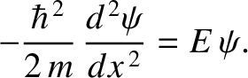 |
(11.64) |
The boundary conditions are
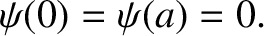 |
(11.65) |
This follows because in the region or , and must be continuous [because a discontinuous
wavefunction would generate a singular term (i.e., the term involving
 ) in the time-independent Schrödinger equation, (11.62),
that could not be balanced, even by an infinite potential].
) in the time-independent Schrödinger equation, (11.62),
that could not be balanced, even by an infinite potential].
Let us search for solutions to Equation (11.64) of the form
 |
(11.66) |
where  is a constant. It follows that
 |
(11.67) |
The solution (11.66) automatically satisfies the boundary condition  . The second boundary
condition,
. The second boundary
condition, 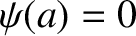 , leads to a quantization of the wavenumber; that is,
 |
(11.68) |
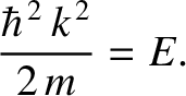
where
 et cetera. (A “quantized” quantity is one that can only take certain discrete values.) According to Equation (11.67), the energy is also quantized.
In fact,
et cetera. (A “quantized” quantity is one that can only take certain discrete values.) According to Equation (11.67), the energy is also quantized.
In fact,  , where
 |
(11.69) |
Thus, the allowed wavefunctions for a particle trapped in a one-dimensional square potential well of infinite depth are
 |
(11.70) |
where  is a positive integer, and
  a constant. We cannot have
  , because, in this case, we obtain
a null wavefunction; that is, , everywhere. Furthermore, if takes a negative integer value
then it generates exactly the same wavefunction as the corresponding positive integer value (assuming
, because, in this case, we obtain
a null wavefunction; that is, , everywhere. Furthermore, if takes a negative integer value
then it generates exactly the same wavefunction as the corresponding positive integer value (assuming
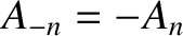 ).
).
The constant , appearing in the previous wavefunction, can be determined from the constraint that the
wavefunction be properly normalized. For the case under consideration, the normalization condition (11.28)
reduces to
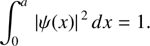 |
(11.71) |
It follows from Equation (11.70) that
 . Hence, the properly normalized version of the wavefunction (11.70)
is
. Hence, the properly normalized version of the wavefunction (11.70)
is
 |
(11.72) |
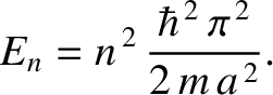
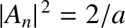
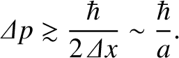
Figure 11.5 shows the first four properly normalized stationary wavefunctions for a particle trapped in a one-dimensional
square potential well of infinite depth; that is,
 ,
for
,
for  to
to  .
.
Figure 11.5:
First four stationary wavefunctions for a particle trapped in a one-dimensional
square potential well of infinite depth.
|
|
The stationary wavefunctions that we have just found are, in essence, standing wave solutions to Schrödinger's equation.
Indeed, the wavefunctions are very similar in form to the classical standing wave solutions discussed in Chapters 4
and 5.
At first sight, it seems rather strange that the lowest possible energy for a particle trapped in a one-dimensional
potential well is not zero, as would be the case in classical mechanics, but rather
 . In fact,
as explained in the following, this residual energy is a direct consequence of Heisenberg's uncertainty principle. A
particle trapped in a one-dimensional well of width
. In fact,
as explained in the following, this residual energy is a direct consequence of Heisenberg's uncertainty principle. A
particle trapped in a one-dimensional well of width  is likely to be found
anywhere inside the well. Thus, the uncertainty in the particle's position is
is likely to be found
anywhere inside the well. Thus, the uncertainty in the particle's position is
 . It
follows from the uncertainty principle, (11.56), that
. It
follows from the uncertainty principle, (11.56), that
 |
(11.73) |
In other words, the particle cannot have zero momentum. In fact, the particle's momentum
must be at least
 .
However, for a free particle,
.
However, for a free particle,
 . Hence, the residual energy associated with the
particle's residual momentum is
. Hence, the residual energy associated with the
particle's residual momentum is
 |
(11.74) |
This type of residual energy, which often occurs in quantum mechanical systems, and has no equivalent in classical
mechanics, is called zero point energy.
![\includegraphics[width=0.9\textwidth]{Chapter11/fig11_05.eps}](img3939.png)