Particle in Finite Square Potential Well

Consider a particle of mass $m$ trapped in a one-dimensional, square, potential well of width $a$ and finite depth $V>0$. Suppose that the potential takes the form

$$U(x) = \left\{ \begin{array}{rll} -V &\mbox{\hspace{0.5cm}}&\... ...\vert\leq a/2\\ [0.5ex] 0&&\mbox{otherwise} \end{array}\right..$$ (11.75)

Here, we have adopted the standard convention that $U(x)\rightarrow 0$ as $\vert x\vert\rightarrow \infty$. This convention is useful because, just as in classical mechanics, a particle whose overall energy, $E$, is negative is bound in the well (i.e., it cannot escape to infinity), whereas a particle whose overall energy is positive is unbound (Fitzpatrick 2012). Because we are interested in bound particles, we shall assume that $E<0$. We shall also assume that $E+V>0$, in order to allow the particle to have a positive kinetic energy inside the well.

Let us search for a stationary state

$$\psi(x,t) = \psi(x)\,{\rm e}^{-{\rm i}\,(E/\hbar)\,t},$$ (11.76)

whose stationary wavefunction, $\psi(x)$, satisfies the time-independent Schrödinger equation, (11.62). Solutions to Equation (11.62) in the symmetric [i.e., $U(-x)=U(x)$] potential (11.75) are either totally symmetric [i.e., $\psi(-x)=\psi(x)$] or totally antisymmetric [i.e., $\psi(-x)=-\psi(x)$]. Moreover, the solutions must satisfy the boundary condition

$$\psi\rightarrow 0 \mbox{\hspace{0.5cm}as\hspace{0.5cm}$\vert x\vert\rightarrow\infty$} ,$$ (11.77)

otherwise they would not correspond to bound states.

Let us, first of all, search for a totally-symmetric solution. In the region to the left of the well (i.e., $x<-a/2$), the solution of the time-independent Schrödinger equation that satisfies the boundary condition $\psi\rightarrow 0$ as $x\rightarrow -\infty$ is

$$\psi(x) = A\,{\rm e}^{\,q\,x},$$ (11.78)

where

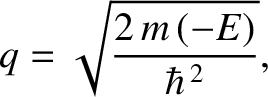$$q = \sqrt{\frac{2\,m\,(-E)}{\hbar^{\,2}}},$$ (11.79)

and $A$ is a constant. By symmetry, the solution in the region to the right of the well (i.e., $x>a/2$) is

$$\psi(x) = A\,{\rm e}^{- q\,x}.$$ (11.80)

The solution inside the well (i.e., $\vert x\vert\leq a/2$) that satisfies the symmetry constraint $\psi(-x)=\psi(x)$ is

$$\psi(x) = B\,\cos(k\,x),$$ (11.81)

where

$$k= \sqrt{\frac{2\,m\,(V+E)}{\hbar^{\,2}}},$$ (11.82)

and $B$ is a constant. The appropriate matching conditions at the edges of the well (i.e., $x=\pm a/2$) are that $\psi(x)$ and $d\psi(x)/dx$ both be continuous [because a discontinuity in the wavefunction, or its first derivative, would generate a singular term in the time-independent Schrödinger equation (i.e., the term involving $d^{\,2}\psi/dx^{\,2}$) that could not be balanced]. The matching conditions yield

$$q = k\,\tan(k\,a/2).$$ (11.83)

Let $y=k\,a/2$. It follows that

$$E = E_0\,y^{\,2} - V,$$ (11.84)

where

$$E_0 = \frac{2\,\hbar^{\,2}}{m\,a^{\,2}}.$$ (11.85)

Moreover, Equation (11.83) becomes

$$\frac{\sqrt{\lambda-y^{\,2}}}{y} = \tan y,$$ (11.86)

with

$$\lambda = \frac{V}{E_0}.$$ (11.87)

Here, $y$ must lie in the range $0<y<\lambda^{1/2}$, in order to ensure that $E$ lies in the range $-V<E<0$.

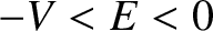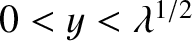
Figure: 11.6 The curves $\tan y$ (solid) and $(\lambda - y^{\,2})^{1/2}/y$ (dashed), calculated for $\lambda = 1.5\,\pi^{\,2}$. The latter curve takes the value 0 when $y>\lambda ^{1/2}$.

The solutions of Equation (11.86) correspond to the intersection of the curve $(\lambda - y^{\,2})^{1/2}/y$ with the curve $\tan y$. Figure 11.6 shows these two curves plotted for a particular value of $\lambda$. In this case, the curves intersect twice, indicating the existence of two totally-symmetric bound states in the well. It is apparent, from the figure, that as $\lambda$ increases (i.e., as the well becomes deeper) there are more and more bound states. However, it is also apparent that there is always at least one totally-symmetric bound state, no matter how small $\lambda$ becomes (i.e., no matter how shallow the well becomes). In the limit $\lambda\gg 1$ (i.e., the limit in which the well is very deep), the solutions to Equation (11.86) asymptote to the roots of $\tan y =\infty$. This gives $y = (2\,n-1)\,\pi/2$, where $n$ is a positive integer, or

$$k = (2\,n-1)\,\frac{\pi}{a}.$$ (11.88)

These solutions are equivalent to the odd-$n$ infinite-depth potential well solutions specified by Equation (11.68).

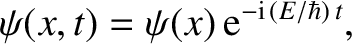
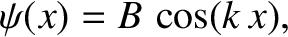
Figure: 11.7 The curves $\tan y$ (solid) and $-y/(\lambda - y^{\,2})^{1/2}$ (dashed), calculated for $\lambda = 1.5\,\pi^{\,2}$.

For the case of a totally-antisymmetric bound state, similar analysis to the preceding yields (see Exercise 12)

$$-\frac{y}{\sqrt{\lambda-y^{\,2}}} = \tan y.$$ (11.89)

The solutions of this equation correspond to the intersection of the curve $\tan y$ with the curve $-y/(\lambda - y^{\,2})^{1/2}$. Figure 11.7 shows these two curves plotted for the same value of $\lambda$ as that used in Figure 11.6. In this case, the curves intersect once, indicating the existence of a single totally-antisymmetric bound state in the well. It is, again, apparent, from the figure, that as $\lambda$ increases (i.e., as the well becomes deeper) there are more and more bound states. However, it is also apparent that when $\lambda$ becomes sufficiently small [i.e., $\lambda < (\pi/2)^2$] then there is no totally antisymmetric bound state. In other words, a very shallow potential well always possesses a totally-symmetric bound state, but does not generally possess a totally-antisymmetric bound state. In the limit $\lambda\gg 1$ (i.e., the limit in which the well becomes very deep), the solutions to Equation (11.89) asymptote to the roots of $\tan y =0$. This gives $y = n\,\pi$, where $n$ is a positive integer, or

$$k= 2\,n\,\frac{\pi}{a}.$$ (11.90)

These solutions are equivalent to the even-$n$ infinite-depth potential well solutions specified by Equation (11.68).

Probably the most surprising aspect of the bound states that we have just described is the possibility of finding the particle outside the well; that is, in the region $\vert x\vert>a/2$ where $U(x)>E$. This follows from Equation (11.80) and (11.81) because the ratio $A/B= \exp(q\,a/2)\,\cos(k\,a/2)$ is not necessarily zero. Such behavior is strictly forbidden in classical mechanics, according to which a particle of energy $E$ is restricted to regions of space where $E>U(x)$ (Fitzpatrick 2012). In fact, in the case of the ground state (i.e., the lowest energy symmetric state) it is possible to demonstrate that the probability of a measurement finding the particle outside the well is (see Exercise 13)

$$P_{\rm out}\simeq 1-2\,\lambda$$ (11.91)

for a shallow well (i.e., $\lambda\ll 1$), and

$$P_{\rm out}\simeq \frac{\pi^{\,2}}{4}\,\frac{1}{\lambda^{\,3/2}}$$ (11.92)

for a deep well (i.e., $\lambda\gg 1$). It follows that the particle is very likely to be found outside a shallow well, and there is a small, but finite, probability of it being found outside a deep well. In fact, the probability of finding the particle outside the well only goes to zero in the case of an infinitely deep well (i.e., $\lambda\rightarrow \infty$).