


Next: Pauli Representation
Up: Spin Angular Momentum
Previous: Spin Space
Since the operators  and
and  commute, they must possess simultaneous
eigenstates (see Sect. 4.10). Let these eigenstates take the form [see Eqs. (556) and (557)]:
commute, they must possess simultaneous
eigenstates (see Sect. 4.10). Let these eigenstates take the form [see Eqs. (556) and (557)]:
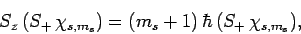
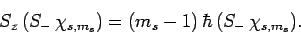
Now, it is easily demonstrated, from the commutation relations (711) and
(712), that
 |
(719) |
and
 |
(720) |
Thus,  and
and  are indeed the raising and lowering operators,
respectively, for spin angular momentum (see Sect. 8.4).
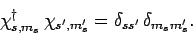
The eigenstates of and are assumed to be orthonormal: i.e.,
are indeed the raising and lowering operators,
respectively, for spin angular momentum (see Sect. 8.4).
The eigenstates of and are assumed to be orthonormal: i.e.,
 |
(721) |
Consider the wavefunction
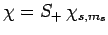 . Since we know,
from Eq. (713), that
. Since we know,
from Eq. (713), that
 , it follows that
 |
(722) |
where use has been made of Eq. (708). Equations (710), (717), (718), and (721)
yield
 |
(723) |
Likewise, if
 then we obtain
 |
(724) |
Assuming that  , the above two inequalities
imply that
, the above two inequalities
imply that
 |
(725) |
Hence, at fixed  , there is both a maximum and a minimum possible value that
  can take.
Let  be the minimum possible value of . It follows
that (see Sect. 8.6)
be the minimum possible value of . It follows
that (see Sect. 8.6)
 |
(726) |
Now, from Eq. (709),
 |
(727) |
Hence,
 |
(728) |
giving
 |
(729) |
Assuming that  , this equation yields
 |
(730) |
Likewise, it is easily demonstrated that
 |
(731) |
Moreover,
 |
(732) |
Now, the raising operator , acting upon  , converts
it into some multiple of
, converts
it into some multiple of  . Employing the raising operator
a second time, we obtain a multiple of
. Employing the raising operator
a second time, we obtain a multiple of  . However, this
process cannot continue indefinitely, since there is a maximum possible
value of . Indeed, after acting upon a sufficient number
of times with the raising operator , we must obtain a multiple
of
. However, this
process cannot continue indefinitely, since there is a maximum possible
value of . Indeed, after acting upon a sufficient number
of times with the raising operator , we must obtain a multiple
of  , so that employing the raising operator one more time
leads to the null state [see Eq. (732)]. If this is not the case then we will inevitably obtain eigenstates
of corresponding to
, so that employing the raising operator one more time
leads to the null state [see Eq. (732)]. If this is not the case then we will inevitably obtain eigenstates
of corresponding to  , which we have already demonstrated is impossible.
It follows, from the above argument, that
 |
(733) |
where  is a positive integer. Hence, the quantum number
can either take positive integer or positive half-integer values.
Up to now, our analysis has been very similar to that which we used earlier to investigate orbital
angular momentum (see Sect. 8). Recall, that for orbital angular momentum the quantum number
is a positive integer. Hence, the quantum number
can either take positive integer or positive half-integer values.
Up to now, our analysis has been very similar to that which we used earlier to investigate orbital
angular momentum (see Sect. 8). Recall, that for orbital angular momentum the quantum number  , which is analogous to ,
is restricted to take integer values (see Cha. 8.5). This implies
that the quantum number
, which is analogous to ,
is restricted to take integer values (see Cha. 8.5). This implies
that the quantum number  , which is analogous to , is also
restricted to take integer values.
However,
the origin of these restrictions is the representation of the orbital
angular momentum operators as differential operators in real space
(see Sect. 8.3). There is no equivalent representation of the
corresponding spin angular momentum operators. Hence, we conclude
that there is no reason why the quantum number cannot take half-integer,
as well as integer, values.
, which is analogous to , is also
restricted to take integer values.
However,
the origin of these restrictions is the representation of the orbital
angular momentum operators as differential operators in real space
(see Sect. 8.3). There is no equivalent representation of the
corresponding spin angular momentum operators. Hence, we conclude
that there is no reason why the quantum number cannot take half-integer,
as well as integer, values.
In 1940, Wolfgang Pauli proved the so-called spin-statistics theorem
using relativistic quantum mechanics. According to this theorem, all
fermions possess half-integer spin (i.e., a half-integer value of ),
whereas all bosons possess integer spin (i.e., an integer value of ). In fact, all presently known
fermions, including electrons and protons, possess spin one-half. In other words,
electrons and protons are characterized by  and
and  .
.
Next: Pauli Representation
Up: Spin Angular Momentum
Previous: Spin Space
Richard Fitzpatrick
2010-07-20