| (246) |
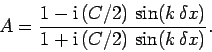 |
(247) |
Listed below is a routine which solves the 1-d advection equation via the Crank-Nicholson method.
// Advect1D.cpp

// Function to evolve advection equation in 1-d:

//  du / dt + v du / dx = 0  for  xl <= x <= xh

//  u = 0  at x=xl and x=xh

// Array u assumed to be of extent N+2.

// Now, ith element of array corresponds to

//  x_i = xl + i * dx    i=0,N+1

// Here, dx = (xh - xl) / (N+1) is grid spacing.

// Function evolves u by single time-step.

// C = v dt / dx, where dt is time-step.

// Uses Crank-Nicholson scheme.

#include <blitz/array.h>

using namespace blitz;

void Tridiagonal (Array<double,1> a, Array<double,1> b, Array<double,1> c,
                  Array<double,1> w, Array<double,1>& u);

void Advect1D (Array<double,1>& u, double C)
{
  // Find N. Declare local arrays.
  int N = u.extent(0) - 2;
  Array<double,1> a(N+2), b(N+2), c(N+2), w(N+2);

  // Initialize tridiagonal matrix
  for (int i = 2; i <= N;   i++) a(i) = - 0.25 * C;
  for (int i = 1; i <= N; i++) b(i) = 1.;
  for (int i = 1; i <= N-1; i++) c(i) = + 0.25 * C;

  // Initialize right-hand side vector
  for (int i = 1; i <= N; i++)
    w(i) = u(i) - 0.25 * C * (u(i+1) - u(i-1));

  // Invert tridiagonal matrix equation
  Tridiagonal (a, b, c, w, u);

  // Calculate i=0 and i=N+1 values
  u(0) = 0.;
  u(N+1) = 0.;
}
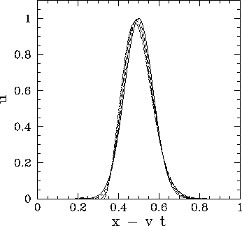
Figure 75 shows an example calculation which uses the above routine to
advect a Gaussian pulse. The initial condition is as specified in Eq. (244),
and the calculation is performed with ![]() ,
,
![]() , and
, and ![]() .
Note that
.
Note that ![]() for these parameters. It can be seen that the pulse propagates at (almost) the
correct speed, and maintains approximately the same shape. Clearly, the
performance of the Crank-Nicholson scheme is vastly superior to that of the Lax scheme.
for these parameters. It can be seen that the pulse propagates at (almost) the
correct speed, and maintains approximately the same shape. Clearly, the
performance of the Crank-Nicholson scheme is vastly superior to that of the Lax scheme.
 |