


Next: The Crank-Nicholson scheme
Up: The wave equation
Previous: The 1-d advection equation
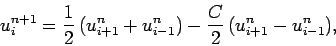
The instability in the differencing scheme (237) can be fixed by replacing
 on the right-hand side by the spatial average of
  taken over the neighbouring grid
points. Thus, we obtain
taken over the neighbouring grid
points. Thus, we obtain
 |
(240) |
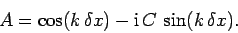
which is known as the Lax scheme. A von Neumann stability analysis
of the Lax scheme yields the following expression for the amplification
factor:
 |
(241) |
Now
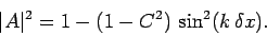 |
(242) |
It follows that the Lax scheme is unconditionally stable (i.e.,  for all
  ), provided that
  . From the definition of
  , the
inequality can also be written
, the
inequality can also be written
 |
(243) |
This is the famous Courant-Friedrichs-Lewy (or CFL) stability criterion.
In fact, all stable explicit differencing schemes for solving the advection equation
are subject to the CFL constraint, which determines the maximum allowable time-step.
Listed below is a routine which solves the 1-d advection equation
via the Lax method.
// Lax1D.cpp

// Function to evolve advection equation in 1-d:

//  du / dt + v du / dx = 0  for  xl <= x <= xh

//  u = 0  at x=xl and x=xh

// Array u assumed to be of extent N+2.

// Now, ith element of array corresponds to

//  x_i = xl + i * dx    i=0,N+1

// Here, dx = (xh - xl) / (N+1) is grid spacing.

// Function evolves u by single time-step.

// C = v dt / dx, where dt is time-step.

// Uses Lax scheme.

#include <blitz/array.h>

using namespace blitz;

void Lax1D (Array<double,1>& u, double C)
{
  // Set N. Declare local array.
  int N = u.extent(0) - 2;
  Array<double,1> u0(N+2);

  // Evolve u
  u0 = u;
  for (int i = 1; i <= N; i++)
    u(i) = 0.5 * (u0(i+1) + u0(i-1)) - 0.5 * C * (u0(i+1) - u0(i-1));

  // Set boundary conditions
  u(0) = 0.;
  u(N+1) = 0.;
}
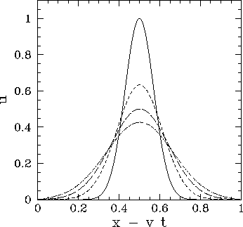
Figure 75 shows an example calculation which uses the above routine to
advect a Gaussian pulse. The initial condition is
![\begin{displaymath}
u(x,0) = \exp[-100\,(x-0.5)^2],
\end{displaymath}](img956.png) |
(244) |
and the calculation is performed with  ,
,
 , and
, and  .
Furthermore,
.
Furthermore,  and
and
 .
Note that
.
Note that  for these parameters. It can be
seen that the pulse is advected at the correct speed: i.e., the
pulse appears approximately stationary when plotted versus
for these parameters. It can be
seen that the pulse is advected at the correct speed: i.e., the
pulse appears approximately stationary when plotted versus  .
Unfortunately, the pulse does not remain the same shape (as it should). Instead, the
pulse becomes gradually lower and wider as it propagates, and eventually
diffuses away entirely.
.
Unfortunately, the pulse does not remain the same shape (as it should). Instead, the
pulse becomes gradually lower and wider as it propagates, and eventually
diffuses away entirely.
Figure 75:
Advection of a 1-d Gaussian pulse.
Numerical calculation performed using
,
, and . The
solid curve shows the initial condition at  , the short-dashed curve the numerical solution
at
, the short-dashed curve the numerical solution
at  , the long-dashed curve the numerical solution
at
, the long-dashed curve the numerical solution
at  , and the dot-dashed curve the numerical solution at
 .
.
 |
It is clear, from the above calculation, that the Lax scheme introduces a spurious
dispersion effect into the advection problem. We can understand the origin
of this effect by attempting a Fourier solution,
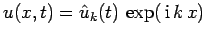 ,
of Eq. (234). We easily obtain
,
of Eq. (234). We easily obtain
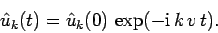 |
(245) |
Note that  is constant in time for all values of . In other words, the
amplitudes of the Fourier harmonics of a true solution of the advection equation
remain constant in time--it is the phases of the harmonics which
evolve. Let us now examine Eq. (242). It can be seen that, provided the CFL condition
is satisfied, the magnitude of the amplification factor,
is constant in time for all values of . In other words, the
amplitudes of the Fourier harmonics of a true solution of the advection equation
remain constant in time--it is the phases of the harmonics which
evolve. Let us now examine Eq. (242). It can be seen that, provided the CFL condition
is satisfied, the magnitude of the amplification factor,  ,
is less than unity for all Fourier harmonics. In other words,
the Lax differencing scheme causes the Fourier harmonics to decay in time. It is this unphysical
attenuation of the Fourier harmonics which gives rise to the strong dispersion effect
illustrated in Fig. 75.
,
is less than unity for all Fourier harmonics. In other words,
the Lax differencing scheme causes the Fourier harmonics to decay in time. It is this unphysical
attenuation of the Fourier harmonics which gives rise to the strong dispersion effect
illustrated in Fig. 75.
Figure 76:
Advection of a 1-d Gaussian pulse.
Numerical calculation performed using
,
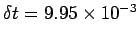 , and . The
dotted curve shows the initial condition at
, and . The
dotted curve shows the initial condition at  , the short-dashed curve the numerical solution
at
, the short-dashed curve the numerical solution
at  , the long-dashed curve the numerical solution
at
, the long-dashed curve the numerical solution
at  , and the solid curve the numerical solution at
 .
.
 |
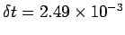
Figure 76 shows a calculation made using the Lax scheme in
which the CFL condition is violated. This
calculation is identical to the one discussed previously, except that the time-step
has been increased to
,
yielding a CFL parameter,  , which exceeds unity. It can be seen that
the pulse grows in amplitude, and eventually starts to break up due to a short-wavelength
instability.
, which exceeds unity. It can be seen that
the pulse grows in amplitude, and eventually starts to break up due to a short-wavelength
instability.
Next: The Crank-Nicholson scheme
Up: The wave equation
Previous: The 1-d advection equation
Richard Fitzpatrick
2006-03-29