The Crank-Nicholson scheme

Let us revisit our temporal differencing scheme:

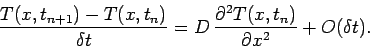$$\frac{T(x,t_{n+1}) - T(x,t_n)}{\delta t} = D \,\frac{\partial^2 T(x,t_n)}{\partial x^2}+ O(\delta t).$$ (210)

Note that the right-hand side is evaluated entirely at the start of the time-step: i.e., at $t_n$. This type of temporal differencing scheme is termed an explicit scheme. Now, explicit schemes are very straightforward to implement, but are also notoriously prone to numerical instabilities. Fortunately, we can often overcome these instabilities by making our differencing scheme implicit in nature. An implicit scheme is one in which the right-hand side is evaluated partly (or wholly) at the end of the time-step: i.e., at $t_{n+1}$. Unfortunately, implicit schemes are generally a great deal more complicated to implement than explicit schemes.

The well-known Crank-Nicholson implicit method for solving the diffusion equation involves taking the average of the right-hand side between the beginning and end of the time-step. In other words,

$$\frac{T(x,t_{n+1}) - T(x,t_n)}{\delta t} = \frac{D}{2} \,\f... ...\,\frac{\partial^2 T(x,t_{n+1})}{\partial x^2}+ O(\delta t)^2.$$ (211)

As indicated by the error term, this method is actually second-order in time.

Adopting our usual spatial differencing scheme, the above expression yields

$$T_i^{n+1} - \frac{C}{2}\,\left(T_{i-1}^{n+1}-2\,T_i^{n+1}+T_... ..._i^n + \frac{C}{2}\,\left(T_{i-1}^n-2\,T_i^n+T_{i+1}^n\right).$$ (212)

When we perform a von Neumann stability analysis of the above scheme, we obtain the following expression for the amplification factor:

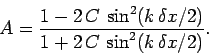$$A = \frac{1 - 2\,C\,\sin^2(k\,\delta x/2)}{1+2\,C\,\sin^2(k\,\delta x/2)}.$$ (213)

Note that $\vert A\vert<1$ for all values of $k$. It follows that the Crank-Nicholson scheme is unconditionally stable. Unfortunately, Eq. (212) constitutes a tridiagonal matrix equation linking the $T_i^{n+1}$ and the $T_i^n$. Thus, the price we pay for the high accuracy and unconditional stability of the Crank-Nicholson scheme is having to invert a tridiagonal matrix equation at each time-step. Usually, this price is well worth paying.