


Next: Sommerfeld Expansion
Up: Quantum Statistics
Previous: Stefan-Boltzmann Law
Conduction Electrons in Metal
The conduction electrons in a metal are non-localized (i.e., they are
not tied to any particular atoms). In conventional metals, each atom contributes
a fixed number of such electrons (corresponding to its valency). To a first approximation, it is possible
to neglect the mutual interaction of the conduction electrons, because this
interaction
is largely shielded out by the stationary ions. The conduction electrons
can, therefore, be treated as an ideal gas. However, the concentration of
such electrons in a metal far exceeds the concentration of
particles in a conventional gas. It is, therefore, not surprising that
conduction electrons cannot normally be analyzed using classical statistics:
in fact, they are subject to Fermi-Dirac statistics
(because electrons are fermions).
Recall, from Section 8.5, that the mean number of particles occupying
state  (energy
 ) is given by
 |
(8.134) |
according to the Fermi-Dirac distribution. Here,
 |
(8.135) |
is termed the Fermi energy of the system. This energy is
determined by the condition that
 |
(8.136) |
where  is the total number of particles contained in the volume
  .
It is clear, from the previous equation, that the Fermi energy,
.
It is clear, from the previous equation, that the Fermi energy,  , is generally
a function of the temperature,
, is generally
a function of the temperature,  .
.
Let us investigate the behavior of the so-called Fermi function,
 |
(8.137) |
as  varies. Here, the energy is measured from
its lowest possible value
varies. Here, the energy is measured from
its lowest possible value
 . If the Fermi energy,
, is
such that
. If the Fermi energy,
, is
such that
 then
then
 ,
and
,
and  reduces to the Maxwell-Boltzmann distribution. However,
for the case of conduction electrons in a metal, we are interested in
the opposite limit, where
reduces to the Maxwell-Boltzmann distribution. However,
for the case of conduction electrons in a metal, we are interested in
the opposite limit, where
 |
(8.138) |
In this limit, if
 then
then
 ,
so that
,
so that
 . On the other hand, if
 then
, so that
then
, so that
![$ F(\epsilon)=
\exp[-\beta (\epsilon-\mu)]$](img2238.png) falls off exponentially with increasing
, just like a classical Maxwell-Boltzmann distribution. Note that
falls off exponentially with increasing
, just like a classical Maxwell-Boltzmann distribution. Note that
 when
when
 . The transition region in which
goes from
a value close to unity to a value close to zero corresponds to an
energy interval of order
. The transition region in which
goes from
a value close to unity to a value close to zero corresponds to an
energy interval of order  , centered on
. In fact,
, centered on
. In fact,  when
when
 , and
, and  when
when
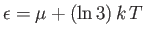 . The behavior of the Fermi function is
illustrated in Figure 8.4.
. The behavior of the Fermi function is
illustrated in Figure 8.4.
Figure 8.4:
The Fermi function.
 |
In the limit as
 , the transition region becomes
infinitesimally narrow. In this case,
, the transition region becomes
infinitesimally narrow. In this case,  for
for
 , and
, and
 for
for
 , as illustrated in Figure 8.4.
This is an obvious result, because when
, as illustrated in Figure 8.4.
This is an obvious result, because when  the conduction
electrons attain their lowest energy, or ground-state, configuration.
Because the Pauli exclusion principle requires that there be no
more than one electron per single-particle quantum state, the lowest
energy configuration is obtained by piling
electrons into the lowest available unoccupied states, until all of
the electrons are used up. Thus, the last electron added to the
pile has a quite considerable energy,
, because all of the
lower energy states are already occupied. Clearly, the exclusion principle
implies that a Fermi-Dirac gas possesses a large mean energy, even at absolute
zero.
the conduction
electrons attain their lowest energy, or ground-state, configuration.
Because the Pauli exclusion principle requires that there be no
more than one electron per single-particle quantum state, the lowest
energy configuration is obtained by piling
electrons into the lowest available unoccupied states, until all of
the electrons are used up. Thus, the last electron added to the
pile has a quite considerable energy,
, because all of the
lower energy states are already occupied. Clearly, the exclusion principle
implies that a Fermi-Dirac gas possesses a large mean energy, even at absolute
zero.
Let us calculate the Fermi energy,  , of a Fermi-Dirac
gas at
. The energy of each particle is related to its
momentum
, of a Fermi-Dirac
gas at
. The energy of each particle is related to its
momentum
 via
via
 |
(8.139) |
where  is the de Broglie wavevector. Here,
  is the electron mass.
At
, all quantum states
whose energy is less than the Fermi energy,
is the electron mass.
At
, all quantum states
whose energy is less than the Fermi energy,  , are filled. The
Fermi energy corresponds to a so-called Fermi momentum,
, are filled. The
Fermi energy corresponds to a so-called Fermi momentum,
 , which
is such that
, which
is such that
 |
(8.140) |
Thus, at
, all quantum states with  are filled, and all
those with
are filled, and all
those with  are empty.
Now, we know, by analogy with Equation (7.183), that there are
 allowable translational states per unit volume of
-space. The volume of
the sphere of radius
allowable translational states per unit volume of
-space. The volume of
the sphere of radius  in
-space is
in
-space is
 . It
follows that the Fermi sphere of radius
contains
. It
follows that the Fermi sphere of radius
contains
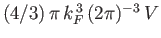 translational states. The number of
quantum states inside the sphere is twice this, because electrons
possess two possible spin states for every possible translational state. Because the
total number of occupied states (i.e., the total number of quantum
states inside the Fermi sphere) must equal the total number of particles
in the gas, it follows that
translational states. The number of
quantum states inside the sphere is twice this, because electrons
possess two possible spin states for every possible translational state. Because the
total number of occupied states (i.e., the total number of quantum
states inside the Fermi sphere) must equal the total number of particles
in the gas, it follows that
 |
(8.141) |
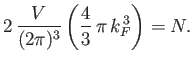
The previous expression can be rearranged to
give
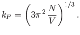 |
(8.142) |
Hence,
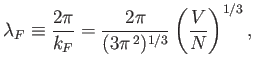 |
(8.143) |
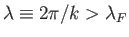
which implies that the de Broglie wavelength,  ,
corresponding to the Fermi energy, is of order the mean separation
between particles
,
corresponding to the Fermi energy, is of order the mean separation
between particles
 . All quantum states with de Broglie
wavelengths
. All quantum states with de Broglie
wavelengths
 are occupied
at
, whereas all those with
are occupied
at
, whereas all those with
 are empty.
According to Equations (8.140) and (8.142), the Fermi energy at
takes the form
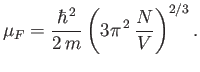 |
(8.144) |
It is easily demonstrated that
 for conventional metals
at room temperature. (See Exercise 17.)
for conventional metals
at room temperature. (See Exercise 17.)
The majority of the conduction electrons in a metal occupy a
band of completely filled states with energies far below the Fermi
energy. In many cases, such electrons have very little effect
on the macroscopic properties of the metal. Consider, for example, the
contribution of the conduction electrons to the specific heat of the metal.
The heat capacity at constant volume,  , of these electrons can
be calculated from a knowledge of their mean energy,
, of these electrons can
be calculated from a knowledge of their mean energy,
 , as a
function of
: that is,
, as a
function of
: that is,
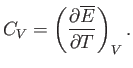 |
(8.145) |
If the electrons obeyed classical Maxwell-Boltzmann statistics, so that
 for all electrons, then the
equipartition theorem would give
for all electrons, then the
equipartition theorem would give
However, the actual situation, in which
has the form shown in Figure 8.4,
is very different. A small change in
does not affect the
mean energies of
the majority of the electrons, with
 , because these electrons
lie in states that are completely filled, and remain so when the temperature
is changed. It follows that these electrons contribute nothing whatsoever to
the heat capacity. On the other hand, the relatively small number of
electrons,
, because these electrons
lie in states that are completely filled, and remain so when the temperature
is changed. It follows that these electrons contribute nothing whatsoever to
the heat capacity. On the other hand, the relatively small number of
electrons,
 , in the energy range of order
, centered on the
Fermi energy, in which
is significantly different from 0 and 1,
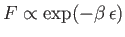
do contribute to the specific heat. In the tail end of this region,
, so the
distribution reverts to a Maxwell-Boltzmann distribution.
Hence, from Equation (8.147),
we expect each electron in this region to contribute roughly an amount
, in the energy range of order
, centered on the
Fermi energy, in which
is significantly different from 0 and 1,
do contribute to the specific heat. In the tail end of this region,
, so the
distribution reverts to a Maxwell-Boltzmann distribution.
Hence, from Equation (8.147),
we expect each electron in this region to contribute roughly an amount
 to the heat capacity. Hence, the heat capacity
can be written
to the heat capacity. Hence, the heat capacity
can be written
 |
(8.148) |
However, because only a fraction  of the total conduction
electrons lie in the tail region of the Fermi-Dirac distribution, we
expect
of the total conduction
electrons lie in the tail region of the Fermi-Dirac distribution, we
expect
 |
(8.149) |
It follows that
 |
(8.150) |
Because
 in conventional metals, the molar specific heat of
the conduction electrons is clearly very much less than the classical value
in conventional metals, the molar specific heat of
the conduction electrons is clearly very much less than the classical value
 . This accounts for the fact that
the molar specific heat capacities of metals at room temperature are
about the same as those of insulators. Before the advent of
quantum mechanics, the classical theory predicted incorrectly that the
presence of conduction electrons should raise the heat capacities of monovalent
metals by 50 percent [i.e.,
] compared to those of insulators.
. This accounts for the fact that
the molar specific heat capacities of metals at room temperature are
about the same as those of insulators. Before the advent of
quantum mechanics, the classical theory predicted incorrectly that the
presence of conduction electrons should raise the heat capacities of monovalent
metals by 50 percent [i.e.,
] compared to those of insulators.
Note that the specific heat (8.150) is not temperature independent.
In fact, using the superscript  to denote the electronic
specific heat, the molar specific heat can be written
to denote the electronic
specific heat, the molar specific heat can be written
 |
(8.151) |
where  is a (positive) constant of proportionality.
At room temperature
is a (positive) constant of proportionality.
At room temperature  is completely masked by the much
larger specific heat,
is completely masked by the much
larger specific heat,  , due to lattice vibrations. However, at
very low temperatures
, due to lattice vibrations. However, at
very low temperatures
 , where
  is a (positive)
constant of proportionality. (See Section 7.14.) Clearly,
at low temperatures,
approaches zero far more rapidly that
the electronic specific heat, as
is reduced. Hence, it should be possible
to measure the electronic contribution to the molar specific
heat at low temperatures.
is a (positive)
constant of proportionality. (See Section 7.14.) Clearly,
at low temperatures,
approaches zero far more rapidly that
the electronic specific heat, as
is reduced. Hence, it should be possible
to measure the electronic contribution to the molar specific
heat at low temperatures.
The total molar specific heat of a metal at low temperatures takes the
form
 |
(8.152) |
Hence,
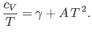 |
(8.153) |
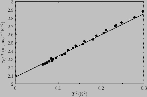
It follows that a plot of  versus
  should yield a
straight-line whose intercept on the vertical axis gives the
coefficient
. Figure 8.5 shows such a plot.
The fact that a good straight-line is obtained verifies that the temperature
dependence of the heat capacity predicted by Equation (8.152) is indeed
correct.
should yield a
straight-line whose intercept on the vertical axis gives the
coefficient
. Figure 8.5 shows such a plot.
The fact that a good straight-line is obtained verifies that the temperature
dependence of the heat capacity predicted by Equation (8.152) is indeed
correct.
Figure:
The low-temperature heat capacity of potassium, plotted as
versus
. The straight-line shows the fit
 . From C. Kittel, and H. Kroemer, Thermal Physics (W.H. Freeman & co., New York NY, 1980).
 |
Next: Sommerfeld Expansion
Up: Quantum Statistics
Previous: Stefan-Boltzmann Law
Richard Fitzpatrick
2016-01-25

