Next: Hydrogen Molecule Ion
Up: Variational Methods
Previous: Variational Principle
A helium atom consists of a nucleus of charge  surrounded
by two electrons. Let us attempt to calculate its ground-state energy.
surrounded
by two electrons. Let us attempt to calculate its ground-state energy.
Let the nucleus lie at the origin of our coordinate
system, and let the position vectors of the two electrons be  and
and  , respectively. The Hamiltonian of the system thus
takes the form
, respectively. The Hamiltonian of the system thus
takes the form
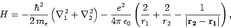 |
(1180) |
where we have neglected any reduced mass effects.
The terms in the above expression represent the kinetic energy of the first
electron, the kinetic energy of the second electron, the electrostatic
attraction between the nucleus and the first electron, the electrostatic
attraction between the nucleus and the second electron, and the
electrostatic repulsion between the two electrons, respectively.
It is the final term which causes all of the difficulties. Indeed, if this
term is neglected then we can write
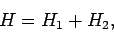 |
(1181) |
where
 |
(1182) |
In other words, the Hamiltonian just becomes the sum of separate Hamiltonians for each electron. In this case, we would expect the
wavefunction to be separable: i.e.,
 |
(1183) |
Hence, Schrödinger's equation
 |
(1184) |
reduces to
 |
(1185) |
where
 |
(1186) |
Of course, Eq. (1185) is the Schrödinger equation of a hydrogen atom whose
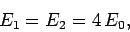
nuclear charge is , instead of  . It follows, from Sect. 9.4 (making the substitution
 ), that if both electrons are in their lowest energy
states then
), that if both electrons are in their lowest energy
states then
where
 |
(1189) |
Here,  is the Bohr radius [see Eq. (679)]. Note that
  is properly normalized. Furthermore,
 |
(1190) |
where
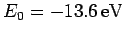 is the hydrogen ground-state
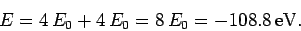
energy [see Eq. (678)]. Thus, our crude estimate
for the ground-state energy of helium becomes
is the hydrogen ground-state
energy [see Eq. (678)]. Thus, our crude estimate
for the ground-state energy of helium becomes
 |
(1191) |
Unfortunately, this estimate is significantly different from the experimentally
determined value, which is
 . This fact
demonstrates that the neglected electron-electron repulsion term makes a
large contribution to the helium ground-state energy.
Fortunately, however, we can use the variational principle to estimate this contribution.
. This fact
demonstrates that the neglected electron-electron repulsion term makes a
large contribution to the helium ground-state energy.
Fortunately, however, we can use the variational principle to estimate this contribution.
Let us employ the separable wavefunction discussed above as our trial
solution. Thus,
![\begin{displaymath}
\psi({\bf r}_1, {\bf r}_2) = \psi_0({\bf r}_1) \psi_0({\bf ...
...{\pi a_0^{ 3}} \exp\left(- \frac{2 [r_1+r_2]}{a_0}\right).
\end{displaymath}](img2726.png) |
(1192) |
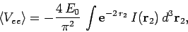
The expectation value of the Hamiltonian (1180) thus becomes
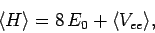 |
(1193) |
where
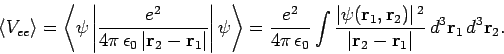 |
(1194) |
The variation principle only guarantees that (1193) yields an
upper bound on the ground-state energy. In reality, we hope
that it will give a reasonably accurate estimate of this energy.
It follows from Eqs. (678), (1192) and (1194) that
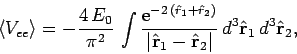 |
(1195) |
where
 . Neglecting the hats, for the sake of clarity, the above
expression can also be written
. Neglecting the hats, for the sake of clarity, the above
expression can also be written
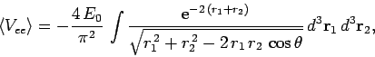 |
(1196) |
where  is the angle subtended between vectors and .
If we perform the integral in space before that in
space then
is the angle subtended between vectors and .
If we perform the integral in space before that in
space then
 |
(1197) |
where
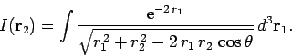 |
(1198) |
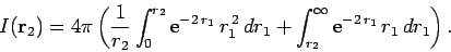
Our first task is to evaluate the function  . Let
. Let
 be a set of spherical polar coordinates in
space whose axis of symmetry runs in the direction of . It follows
that
be a set of spherical polar coordinates in
space whose axis of symmetry runs in the direction of . It follows
that
 . Hence,
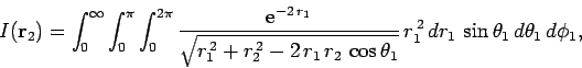 |
(1199) |
which trivially reduces to
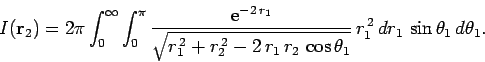 |
(1200) |
Making the substitution
 , we can see that
 |
(1201) |
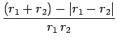
Now,
giving
 |
(1203) |
But,
yielding
![\begin{displaymath}
I({\bf r}_2) = \frac{\pi}{r_2}\left[1-{\rm e}^{-2 r_2} (1+r_2)\right].
\end{displaymath}](img2750.png) |
(1206) |
Since the function only depends on the magnitude of ,
the integral (1197) reduces to
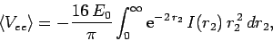 |
(1207) |
which yields
![\begin{displaymath}
\langle V_{ee}\rangle = -16 E_0\int_{0}^\infty
{\rm e}^{-2\...
...{\rm e}^{-2 r_2} (1+r_2)\right]r_2 dr_2=
-\frac{5}{2} E_0.
\end{displaymath}](img2752.png) |
(1208) |
Hence, from (1193), our estimate for the ground-state
energy of helium is
 |
(1209) |
This is remarkably close to the correct result.
We can actually refine our estimate further. The trial wavefunction (1192) essentially treats the two electrons as
non-interacting particles. In
reality, we would expect one electron to partially shield the nuclear
charge from the other, and vice versa. Hence, a better
trial wavefunction might be
![\begin{displaymath}
\psi({\bf r}_1, {\bf r}_2) =
\frac{Z^3}{\pi a_0^{ 3}} \exp\left(- \frac{Z [r_1+r_2]}{a_0}\right),
\end{displaymath}](img2754.png) |
(1210) |
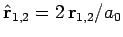
where  is effective nuclear charge number seen by each
electron. Let us recalculate the ground-state energy of helium
as a function of
is effective nuclear charge number seen by each
electron. Let us recalculate the ground-state energy of helium
as a function of  , using the above trial wavefunction, and then
minimize the result with respect to . According to
the variational principle, this should give us an even better estimate
for the ground-state energy.
, using the above trial wavefunction, and then
minimize the result with respect to . According to
the variational principle, this should give us an even better estimate
for the ground-state energy.
We can rewrite the expression (1180) for the Hamiltonian
of the helium atom in the form
 |
(1211) |
where
 |
(1212) |
is the Hamiltonian of a hydrogen atom with nuclear charge  ,
,
 |
(1213) |
is the electron-electron repulsion term, and
![\begin{displaymath}
U(Z) = \frac{e^2}{4\pi \epsilon_0}\left(\frac{[Z-2]}{r_1} + \frac{[Z-2]}{r_2}\right).
\end{displaymath}](img2760.png) |
(1214) |
It follows that
 |
(1215) |
where
 is the ground-state energy of a hydrogen
atom with nuclear charge ,
is the ground-state energy of a hydrogen
atom with nuclear charge ,
 is the value of the electron-electron repulsion term when
recalculated with the wavefunction (1210) [actually, all we
need to do is to make the substitution
is the value of the electron-electron repulsion term when
recalculated with the wavefunction (1210) [actually, all we
need to do is to make the substitution
 ], and
 |
(1216) |
Here,
 is the expectation value of
  calculated
for a hydrogen atom with nuclear charge . It follows from
Eq. (695) [with
calculated
for a hydrogen atom with nuclear charge . It follows from
Eq. (695) [with  , and making the substitution
 ] that
 |
(1217) |
Hence,
 |
(1218) |
since
 .
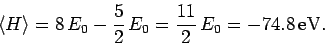
Collecting the various terms, our new expression for the expectation
value of the Hamiltonian becomes
.
Collecting the various terms, our new expression for the expectation
value of the Hamiltonian becomes
![\begin{displaymath}
\langle H\rangle(Z) = \left[2 Z^2 - \frac{5}{4} Z - 4 Z (Z-2)\right] E_0
= \left[-2 Z^2+ \frac{27}{4} Z\right] E_0.
\end{displaymath}](img2771.png) |
(1219) |
The value of which minimizes this expression is the root of
![\begin{displaymath}
\frac{d\langle H\rangle}{dZ} = \left[-4 Z+ \frac{27}{4}\right] E_0 = 0.
\end{displaymath}](img2772.png) |
(1220) |
It follows that
 |
(1221) |
The fact that confirms our earlier conjecture that the electrons partially
shield the nuclear charge from one another. Our new estimate
for the ground-state energy of helium is
 |
(1222) |
This is clearly an improvement on our previous estimate (1209) [recall that the
correct result is  eV].
eV].
Obviously, we could get even closer to the correct value of the
helium ground-state energy by using a
more complicated trial wavefunction with more adjustable parameters.
Note, finally, that since the two electrons in a helium atom are indistinguishable fermions, the overall wavefunction must be anti-symmetric with respect to exchange of particles (see Sect. 6).
Now, the overall wavefunction is the product of the spatial wavefunction
and the spinor representing the spin-state. Our spatial wavefunction (1210) is obviously symmetric with respect to exchange of
particles. This means that the spinor must be anti-symmetric.
It is clear, from Sect. 11.4, that if the spin-state of
an  system consisting of two spin one-half particles (i.e., two electrons)
is anti-symmetric with respect to interchange of particles then the system is
in the so-called singlet state with overall spin zero. Hence,
the ground-state of helium has overall electron spin zero.
system consisting of two spin one-half particles (i.e., two electrons)
is anti-symmetric with respect to interchange of particles then the system is
in the so-called singlet state with overall spin zero. Hence,
the ground-state of helium has overall electron spin zero.
Next: Hydrogen Molecule Ion
Up: Variational Methods
Previous: Variational Principle
Richard Fitzpatrick
2010-07-20
![$\displaystyle \left[\frac{\sqrt{r_1^{ 2}+r_2^{ 2}-2 r_1 r_2 \mu}}{r_1 r_2}\right]_{+1}^{-1}$](img2742.png)