


Next: Scattering Theory
Up: Variational Methods
Previous: Helium Atom
The hydrogen molecule ion consists of an electron orbiting about
two protons, and is the simplest imaginable molecule. Let us
investigate whether or not this molecule possesses a bound state: i.e., whether or
not it possesses a ground-state whose energy is less than that of
a hydrogen atom and a free proton.
According
to the variation principle, we can deduce that the  ion has a bound state if we can find any
trial wavefunction for which the total Hamiltonian of the system has an expectation value less than that of a hydrogen atom and a free proton.
ion has a bound state if we can find any
trial wavefunction for which the total Hamiltonian of the system has an expectation value less than that of a hydrogen atom and a free proton.
Figure 26:
The hydrogen molecule ion.
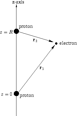 |
Suppose that the two protons are separated by a distance  . In fact, let them lie on the
  -axis, with the first at the origin, and
the second at
-axis, with the first at the origin, and
the second at  (see Fig. 26). In the following, we shall treat the
protons as essentially stationary. This is reasonable, since the electron
moves far more rapidly than the protons.
(see Fig. 26). In the following, we shall treat the
protons as essentially stationary. This is reasonable, since the electron
moves far more rapidly than the protons.
Let us try
![\begin{displaymath}
\psi({\bf r})_\pm = A\left[\psi_0({\bf r}_1) \pm \psi_0({\bf r}_2)\right]
\end{displaymath}](img2779.png) |
(1223) |
as our trial wavefunction, where
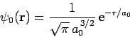 |
(1224) |
is a normalized hydrogen ground-state wavefunction centered on the origin, and  are
the position vectors of the electron with respect to each of the protons
(see Fig. 26). Obviously, this is a very simplistic wavefunction,
since it is just a linear combination of hydrogen ground-state
wavefunctions centered on each proton. Note, however, that the wavefunction respects
the obvious symmetries in the problem.
are
the position vectors of the electron with respect to each of the protons
(see Fig. 26). Obviously, this is a very simplistic wavefunction,
since it is just a linear combination of hydrogen ground-state
wavefunctions centered on each proton. Note, however, that the wavefunction respects
the obvious symmetries in the problem.
Our first task is to normalize our trial wavefunction. We require that
 |
(1225) |
Hence, from (1223),
 , where
![\begin{displaymath}
I = \int\left[\vert\psi_0({\bf r}_1)\vert^2 + \vert\psi_0({\...
...2 \pm
2 \psi_0({\bf r}_1) \psi({\bf r}_2)\right] d^3{\bf r}.
\end{displaymath}](img2784.png) |
(1226) |
It follows that
 |
(1227) |
with
 |
(1228) |
Let us employ the standard spherical polar coordinates ( ,
,  ,
,  ).
Now, it is easily seen that
).
Now, it is easily seen that  and
and
 . Hence,
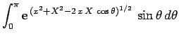
![\begin{displaymath}
J = 2\int_0^\infty \int_0^\pi \exp\left[-x-(x^2+X^2-2 x X \cos\theta)^{1/2}\right] x^2 dx \sin\theta d\theta,
\end{displaymath}](img2789.png) |
(1229) |
where  . Here, we have already performed the trivial integral.
Let
. Here, we have already performed the trivial integral.
Let
 . It follows that
 , giving
Thus,
which evaluates to
 |
(1232) |
Now, the Hamiltonian of the electron is written
 |
(1233) |
Note, however, that
 |
(1234) |
since
 are hydrogen ground-state wavefunctions.
It follows that
are hydrogen ground-state wavefunctions.
It follows that
Hence,
 |
(1236) |
where
Now,
 |
(1239) |
which reduces to
 |
(1240) |
giving
![\begin{displaymath}
D = \frac{1}{X} \left( 1-[1+X] {\rm e}^{-2 X}\right).
\end{displaymath}](img2813.png) |
(1241) |
Furthermore,
![\begin{displaymath}
E = 2\int_0^\infty \int_0^\pi \exp\left[-x-(x^2+X^2-2 x X \cos\theta)^{1/2}\right] x dx \sin\theta d\theta,
\end{displaymath}](img2814.png) |
(1242) |
which reduces to
yielding
 |
(1244) |
Our expression for the expectation value of the electron Hamiltonian is
![\begin{displaymath}
\langle H\rangle = \left[1+ 2 \frac{(D\pm E)}{(1\pm J)}\right] E_0,
\end{displaymath}](img2818.png) |
(1245) |
where  ,
,  , and
, and  are specified as functions of in
Eqs. (1232), (1241), and (1244), respectively.
In order
to obtain the total energy of the molecule, we must add to this the
potential energy of the two protons. Thus,
are specified as functions of in
Eqs. (1232), (1241), and (1244), respectively.
In order
to obtain the total energy of the molecule, we must add to this the
potential energy of the two protons. Thus,
 |
(1246) |
since
 .
Hence, we can write
.
Hence, we can write
 |
(1247) |
where  is the hydrogen ground-state energy, and
![\begin{displaymath}
F_\pm(X) = -1 + \frac{2}{X}\left[\frac{(1+X) {\rm e}^{-2 X...
...X^2/3)
{\rm e}^{-X}}{1\pm (1+X+X^2/3) {\rm e}^{-X}}\right].
\end{displaymath}](img2822.png) |
(1248) |
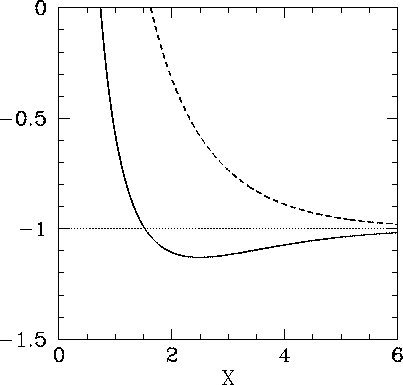
The functions  and
and  are both plotted in Fig. 27.
Recall that in order for the ion to be in a bound state it must have a lower
energy than a hydrogen atom and a free proton: i.e.,
are both plotted in Fig. 27.
Recall that in order for the ion to be in a bound state it must have a lower
energy than a hydrogen atom and a free proton: i.e.,
 . It follows from Eq. (1247) that a bound state
corresponds to
. It follows from Eq. (1247) that a bound state
corresponds to  . Clearly, the even trial wavefunction
  possesses a bound state, whereas the odd trial wavefunction
  does not [see Eq. (1223)]. This is hardly surprising, since the
even wavefunction maximizes the electron probability density between
the two protons, thereby reducing their mutual electrostatic repulsion. On the other hand, the odd
wavefunction does exactly the opposite. The binding energy of the
ion is defined as the difference between its energy and that of a
hydrogen atom and a free proton: i.e.,
does not [see Eq. (1223)]. This is hardly surprising, since the
even wavefunction maximizes the electron probability density between
the two protons, thereby reducing their mutual electrostatic repulsion. On the other hand, the odd
wavefunction does exactly the opposite. The binding energy of the
ion is defined as the difference between its energy and that of a
hydrogen atom and a free proton: i.e.,
 |
(1249) |
According to the variational principle, the binding energy is less than or
equal to the minimum binding energy which can be inferred from Fig. 27.
This minimum occurs when  and
and
 .
Thus, our estimates for the separation between the two
protons, and the binding energy, for the ion
are
.
Thus, our estimates for the separation between the two
protons, and the binding energy, for the ion
are
 and
and
 eV, respectively. The experimentally
determined values are
eV, respectively. The experimentally
determined values are
 m, and
  eV, respectively. Clearly, our estimates are not particularly accurate. However,
our calculation does establish, beyond any doubt, the existence of
a bound state of the ion, which is all that we set out to achieve.
eV, respectively. Clearly, our estimates are not particularly accurate. However,
our calculation does establish, beyond any doubt, the existence of
a bound state of the ion, which is all that we set out to achieve.
Figure 27:
The functions (solid curve) and (dashed curve).
 |
Next: Scattering Theory
Up: Variational Methods
Previous: Helium Atom
Richard Fitzpatrick
2010-07-20
![$\displaystyle - \frac{1}{x X}\left[{\rm e}^{-(x+X)} (1+x+X) - {\rm e}^{-\vert x-X\vert} (1+\vert x-X\vert)\right].$](img2795.png)
![$\displaystyle - \frac{2}{X} {\rm e}^{-X}\int_0^X \left[{\rm e}^{-2 x} (1+X+x)-
(1+X-x)\right]x dx$](img2797.png)
![$\displaystyle -\frac{2}{X}\int_X^\infty {\rm e}^{-2 x}\left[{\rm e}^{-X} (1+X+x)-
{\rm e}^X (1-X+x)\right] x dx,$](img2798.png)
![$\displaystyle A\left[-\frac{\hbar^2}{2 m_e} \nabla^2 - \frac{e^2}{4\pi \epsi...
...frac{1}{r_2}\right)\right]
\left[\psi_0({\bf r}_1) \pm \psi_0({\bf r}_2)\right]$](img2804.png)
![$\displaystyle E_0 \psi - A \left(\frac{e^2}{4\pi \epsilon_0}\right)\left[
\frac{\psi_0({\bf r}_1)}{r_2}\pm \frac{\psi_0({\bf r}_2)}{r_1}\right].$](img2805.png)
![$\displaystyle - \frac{2}{X} {\rm e}^{-X}\int_0^X \left[{\rm e}^{-2 x} (1+X+x)-
(1+X-x)\right]dx$](img2815.png)
![$\displaystyle -\frac{2}{X}\int_X^\infty {\rm e}^{-2 x}\left[{\rm e}^{-X} (1+X+x)-
{\rm e}^X (1-X+x)\right] dx,$](img2816.png)