


Next: Sudden Perturbations
Up: Time-Dependent Perturbation Theory
Previous: Nuclear Magnetic Resonance
Let us now try to find approximate solutions to Equation (8.11) for a general
system. It is convenient to work in terms of the time evolution
operator,  , which is defined
 |
(8.37) |
(See Section 3.2.)
As before,
 is the state ket of the
system at time
is the state ket of the
system at time  , given that the state ket at the initial
time
, given that the state ket at the initial
time  is
is  . It is easily seen that the time evolution operator
satisfies the differential equation
. It is easily seen that the time evolution operator
satisfies the differential equation
 |
(8.38) |
subject to the initial condition
 |
(8.39) |
(See Section 3.2.)
In the absence of the external perturbation, the time evolution operator
reduces to
![$\displaystyle T(t_0, t) = \exp\left[\frac{-{\rm i} \, H_0\,(t-t_0)}{\hbar}\right].$](img2332.png) |
(8.40) |
Let us switch on the perturbation, and look for a solution of the
form
![$\displaystyle T(t_0, t) = \exp\left[\frac{ -{\rm i} \, H_0\,(t-t_0)}{\hbar}\right] T_I(t_0, t).$](img2333.png) |
(8.41) |
It is readily demonstrated that
 satisfies the differential
equation
satisfies the differential
equation
 |
(8.42) |
where
![$\displaystyle H_I(t_0,t) = \exp\left[\frac{\,{\rm i} \, H_0\,(t-t_0)}{\hbar}\right] H_1 \exp\left[\frac{ -{\rm i} \, H_0\,(t-t_0)}{\hbar}\right],$](img2336.png) |
(8.43) |
subject to the initial condition
 |
(8.44) |
(See Exercise 3.)
Note that  specifies that component of the time evolution operator
that is generated by the time-dependent perturbation. Thus, we would expect
to contain all of the information regarding transitions between different
eigenstates of
specifies that component of the time evolution operator
that is generated by the time-dependent perturbation. Thus, we would expect
to contain all of the information regarding transitions between different
eigenstates of  caused by the perturbation.
Suppose that the system starts off at time
in the eigenstate  of
the unperturbed Hamiltonian. The subsequent evolution of
the state ket is given by Equation (8.6),
of
the unperturbed Hamiltonian. The subsequent evolution of
the state ket is given by Equation (8.6),
![$\displaystyle \vert i, t_0, t\rangle = \sum_f c_f(t) \exp\left[\frac{ -{\rm i} \, E_f\,(t-t_0)}{\hbar}\right] \vert f\rangle.$](img2339.png) |
(8.45) |
However, we also have
![$\displaystyle \vert i, t_0, t\rangle = \exp\left[\frac{-{\rm i} \, H_0\,(t-t_0)}{\hbar}\right] T_I(t_0, t)\, \vert i\rangle.$](img2340.png) |
(8.46) |
It follows that
 |
(8.47) |
where use has been made of
 .
Thus, the probability that the system is found in some final state
.
Thus, the probability that the system is found in some final state  at time
, given that it was definitely in the initial state
at time
,
is simply
at time
, given that it was definitely in the initial state
at time
,
is simply
 |
(8.48) |
This quantity is usually termed the transition probability
between states
and
.
Note that the differential equation (8.45), plus the initial condition
(8.47), are equivalent to the following integral equation:
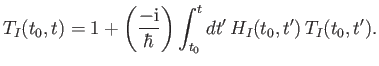 |
(8.49) |
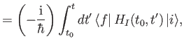
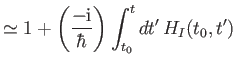
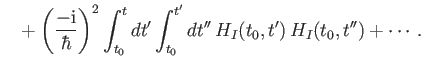
We can obtain an approximate solution to this equation via iteration:
This expansion is known as the Dyson series [34].
Let
 |
(8.51) |
where the superscript  refers to a first-order term in the expansion,
et cetera. It follows from Equations (8.50) and (8.53) that
refers to a first-order term in the expansion,
et cetera. It follows from Equations (8.50) and (8.53) that
These expressions simplify to give
where
 |
(8.58) |
and
 |
(8.59) |
Here, use has been made of the completeness relation
 , where the
sum is over all energy eigenstates.
The transition probability between states
, where the
sum is over all energy eigenstates.
The transition probability between states  and
and  is
simply
is
simply
 |
(8.60) |
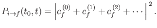
According to the previous analysis, there is no possibility of a
transition between the initial state,
, and the final state,
, (where  )
to zeroth order (i.e., in the absence of the perturbation). To
first order, the transition probability is proportional to
the time integral of the matrix element
)
to zeroth order (i.e., in the absence of the perturbation). To
first order, the transition probability is proportional to
the time integral of the matrix element
 ,
weighted by an oscillatory phase-factor. Thus, if the matrix
element is zero then there is no chance of a first-order transition between
states
and
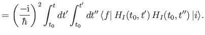
. However, to second order,
a transition between states
and
is possible
even when the
matrix element
is zero.
,
weighted by an oscillatory phase-factor. Thus, if the matrix
element is zero then there is no chance of a first-order transition between
states
and
. However, to second order,
a transition between states
and
is possible
even when the
matrix element
is zero.
Next: Sudden Perturbations
Up: Time-Dependent Perturbation Theory
Previous: Nuclear Magnetic Resonance
Richard Fitzpatrick
2016-01-22
![$\displaystyle \simeq 1 +\left( \frac{-{\rm i}}{\hbar}\right) \int_{t_0}^t dt'\,...
...rm i}}{\hbar}\right) \int_{t_0}^{t'} dt''\,H_I(t_0, t'')\, T_I(t_0, t'')\right]$](img2346.png)
![$\displaystyle = \left(\frac{-{\rm i}}{\hbar}\right) \int_{t_0}^t dt'\, \exp[\,{\rm i} \,\omega_{fi}\, (t'-t_0)]\, H_{fi}(t') ,$](img2357.png)
![$\displaystyle = \left(\frac{-{\rm i}}{\hbar}\right)^2 \sum_m \int_{t_0}^t dt'\int_{t_0}^{t' }dt''\,\exp[\,{\rm i} \,\omega_{fm}\,(t'-t_0)]\, H_{fm}(t')$](img2358.png)