Next: Ray Tracing Up: Waves in Inhomogeneous Plasmas Previous: Collisional Damping Contents
 -direction, is launched along the
  -axis, from
an antenna located at large positive , and reflected from a cutoff located
at
-axis, from
an antenna located at large positive , and reflected from a cutoff located
at  . Up to now, we have only considered infinite wave-trains, characterized
by a discrete frequency,
. Up to now, we have only considered infinite wave-trains, characterized
by a discrete frequency,  . Let us now consider the more realistic
case in which the antenna emits a finite pulse of radio waves.
. Let us now consider the more realistic
case in which the antenna emits a finite pulse of radio waves.
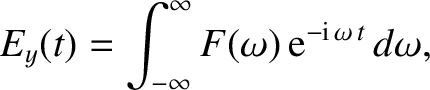
The pulse structure is conveniently represented as
where is the electric field produced by
the antenna, which is assumed to lie at
is the electric field produced by
the antenna, which is assumed to lie at  .
Suppose that the pulse is a signal of roughly constant (angular)
frequency
.
Suppose that the pulse is a signal of roughly constant (angular)
frequency  ,
which lasts a time
,
which lasts a time  , where is long compared to
 . It
follows that
. It
follows that  possesses narrow maxima around
 . In other words,
only those frequencies that lie very close to the central
frequency, , play a significant role in the propagation of the pulse.
. In other words,
only those frequencies that lie very close to the central
frequency, , play a significant role in the propagation of the pulse.
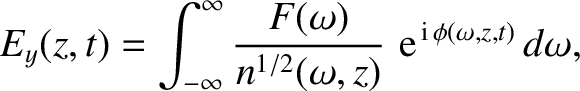
Each component frequency of the pulse yields a wave that
propagates independently along the -axis, in a manner specified by the
appropriate WKB solution [see Equations (6.17) and (6.18)]. Thus, if Equation (6.70)
specifies the signal at the antenna (i.e., at
) then the signal at coordinate (where
 )
is given by
)
is given by
 |
(6.72) |
 .
.
Equation (6.71) can be regarded as a contour integral in -space.
The quantity  is a relatively slowly varying function of
, whereas the phase,
is a relatively slowly varying function of
, whereas the phase,  , is a large and rapidly varying
function of .
The rapid
oscillations of
, is a large and rapidly varying
function of .
The rapid
oscillations of
 over most of the path of
integration ensure that the integrand averages almost to zero. However,
this cancellation argument does not apply to places on the
integration path where the phase
is stationary: that is,
places where
over most of the path of
integration ensure that the integrand averages almost to zero. However,
this cancellation argument does not apply to places on the
integration path where the phase
is stationary: that is,
places where
 has an extremum. The integral can, therefore, be
estimated by finding those points where
has a vanishing derivative,
evaluating (approximately) the integral in the neighborhood of each of
these points, and summing the contributions. This procedure is called
the method of stationary phase (Budden 1985).
has an extremum. The integral can, therefore, be
estimated by finding those points where
has a vanishing derivative,
evaluating (approximately) the integral in the neighborhood of each of
these points, and summing the contributions. This procedure is called
the method of stationary phase (Budden 1985).
Suppose that
has a vanishing first derivative
at
 . In the neighborhood of this point,
can be expanded as a Taylor series,
. In the neighborhood of this point,
can be expanded as a Taylor series,
 |
(6.73) |
 is used to indicate or its
second derivative evaluated at
. Because
is used to indicate or its
second derivative evaluated at
. Because
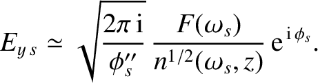
 is slowly varying, the contribution to the integral from this
stationary phase point is approximately
is slowly varying, the contribution to the integral from this
stationary phase point is approximately
![$\displaystyle E_{y\,s} \simeq \frac{F(\omega_s) \,{\rm e}^{\,{\rm i}\,\phi_s}}{...
...nfty} \exp\left[\frac{\rm i}{2}\,\phi_s''\,(\omega-\omega_s)^{2}\right]d\omega.$](img2074.png) |
(6.74) |
![$\displaystyle E_{y\,s}\simeq \frac{F(\omega_s) \,{\rm e}^{\,{\rm i}\,\phi_s}}{n...
...cos\left(\pi \,t^{2}/2\right)+{\rm i}\,\sin\left(\pi\, t^{2}/2\right)\right]dt,$](img2075.png) |
(6.75) |
 |
(6.76) |
 |
(6.77) |
Integrals of the form (6.71) can be calculated exactly using the
method of steepest descent (Brillouin 1960; Budden 1985). The stationary
phase approximation (6.78) agrees with the leading term of the
method of steepest descent (which is far more difficult to implement
than the method of stationary phase) provided that
is
real (i.e., provided that
the stationary point lies on the real axis). If is complex, however, then the stationary phase
method can yield erroneous results.
It follows, from the previous discussion,
that the right-hand side of Equation (6.71) averages to a very small
value, expect
for those special values of and  at which one of the points of stationary
phase in -space coincides with one of the peaks of . The
locus of these special values of and can obviously be regarded as the
equation of motion of the pulse as it propagates along the -axis. Thus, the equation of motion is
specified by
at which one of the points of stationary
phase in -space coincides with one of the peaks of . The
locus of these special values of and can obviously be regarded as the
equation of motion of the pulse as it propagates along the -axis. Thus, the equation of motion is
specified by
 |
(6.79) |
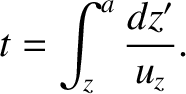
Suppose that the -velocity of a pulse of central frequency
at coordinate is given by
 . The differential
equation of motion of the pulse is then
. The differential
equation of motion of the pulse is then
 . This can be integrated,
using the boundary condition at
. This can be integrated,
using the boundary condition at  , to give the full equation
of motion:
, to give the full equation
of motion:
 is usually called the
group-velocity. It is easily demonstrated that
the previous expression for the group-velocity is
entirely consistent with that
given in Equation (5.72).
is usually called the
group-velocity. It is easily demonstrated that
the previous expression for the group-velocity is
entirely consistent with that
given in Equation (5.72).
The dispersion relation for an electromagnetic plasma wave propagating through an unmagnetized plasma is [see Equation (6.121)]
Here, we have assumed that equilibrium quantities are functions of only,
and that the wave propagates along the -axis.
The phase-velocity
of waves of frequency
propagating along the -axis is given
by
According to Equations (6.82) and (6.83), the corresponding group-velocity
is
It follows that
 |
(6.86) |
 ,
and
,
and
 for
for  , which implies
that the reflection point corresponds to .
It is clear from Equations (6.84) and (6.85) that the phase-velocity of the wave is always greater than the velocity of
light in vacuum, whereas the group-velocity is always less than this
velocity.
Furthermore, as the reflection point, , is approached from positive ,
the phase-velocity tends to infinity, whereas the group-velocity tends
to zero.
, which implies
that the reflection point corresponds to .
It is clear from Equations (6.84) and (6.85) that the phase-velocity of the wave is always greater than the velocity of
light in vacuum, whereas the group-velocity is always less than this
velocity.
Furthermore, as the reflection point, , is approached from positive ,
the phase-velocity tends to infinity, whereas the group-velocity tends
to zero.
Although we have only analyzed the motion of the
pulse as it travels from the antenna to the reflection point, it is
easily demonstrated that the speed of the reflected pulse at position
is the same as that of the incident pulse. In other words, the group velocities
of pulses traveling in opposite directions are of equal magnitude.
![$\displaystyle t = \frac{1}{c} \int_z^a \left[\frac{\partial(\omega \,n)}{\partial\omega}
\right]_{\omega=\omega_0} dz'.$](img2080.png)
![$\displaystyle u_z(\omega_0,z) = c\left/ \left(\frac{\partial[\omega \,n(\omega,z)]}{\partial\omega}
\right)_{\omega=\omega_0}\right..$](img2084.png)
![$\displaystyle n(\omega,z) = \left[1-\frac{{\mit\Pi}_e^{2}(z)}{\omega^2}\right]^{1/2}.$](img2086.png)
![$\displaystyle v_z(\omega,z) = \frac{c}{n(\omega,z)} = c\left[1-\frac{{\mit\Pi}_e^{2}(z)}{\omega^2}\right]^{-1/2}.$](img2087.png)
![$\displaystyle u_z(\omega,z) = c \left[1-\frac{{\mit\Pi}_e^{2}(z)}{\omega^2}\right]^{1/2}.$](img2088.png)