Next: Nonlinear Tearing Mode Theory
Up: Magnetohydrodynamic Fluids
Previous: Magnetic Reconnection
Linear Tearing Mode Theory
Consider the interface between two plasmas containing magnetic fields of
different orientations. The simplest imaginable field configuration is that
illustrated in Figure 7.7. Here, the field varies in the  -direction, and
is parallel to the
-direction, and
is parallel to the  -axis. The field is directed in the
 -direction for
  , and in the
  -direction for
  . The interface
is situated at
. The interface
is situated at  . The sudden reversal of the field direction across the
interface gives rise to a
. The sudden reversal of the field direction across the
interface gives rise to a  -directed current sheet at
.
-directed current sheet at
.
Figure 7.7:
A reconnecting magnetic field configuration.
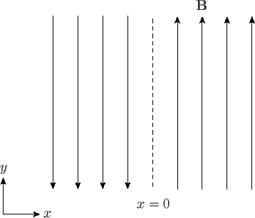 |
With the neglect of plasma resistivity, the field configuration shown in Figure 7.7
represents a stable equilibrium state, assuming, of course,
that we have normal pressure balance
across the interface. But, does the field configuration remain stable when we take
resistivity into account? If not, then we expect an instability to develop that relaxes the
configuration to one possessing lower magnetic energy. As we shall see, this
type of relaxation process inevitably entails the breaking and reconnection of magnetic
field-lines, and is, therefore, termed magnetic reconnection. The
magnetic energy released during the reconnection process eventually appears as
plasma thermal
energy. Thus, magnetic reconnection also involves plasma heating.
In the following, we shall outline the standard method for determining the
linear stability of the type of magnetic field configuration
shown in Figure 7.7, taking into account the effect of plasma resistivity.
We are particularly
interested in plasma instabilities that are stable in the absence of resistivity,
and only grow when the resistivity is non-zero. Such instabilities are
conventionally termed tearing modes.
Because magnetic reconnection is, in fact, a nonlinear process, we shall
then proceed to investigate the nonlinear development of tearing modes.
The equilibrium magnetic field is written
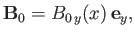 |
(7.171) |
where
 .
There is assumed to be no equilibrium plasma flow. The linearized
equations of resistive-MHD [i.e., Equations (7.1)-(7.4), with Equation (7.3) replaced by Equation (7.102)], assuming incompressible flow, take the form
.
There is assumed to be no equilibrium plasma flow. The linearized
equations of resistive-MHD [i.e., Equations (7.1)-(7.4), with Equation (7.3) replaced by Equation (7.102)], assuming incompressible flow, take the form
Here,  is the equilibrium plasma density,
  the
perturbed magnetic field,
the
perturbed magnetic field,  the perturbed plasma velocity,
 the perturbed plasma pressure, and use has been made of Maxwell's equation. The assumption of incompressible
plasma flow is valid provided that the plasma velocity associated with the
instability remains significantly
smaller than both the Alfvén velocity and the sonic velocity.
the perturbed plasma pressure, and use has been made of Maxwell's equation. The assumption of incompressible
plasma flow is valid provided that the plasma velocity associated with the
instability remains significantly
smaller than both the Alfvén velocity and the sonic velocity.
Suppose that all perturbed quantities vary like
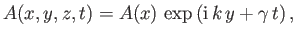 |
(7.176) |
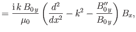
where  is the instability growth-rate. The
-component of
Equation (7.172), and the
-component of the curl of Equation (7.173),
reduce to
is the instability growth-rate. The
-component of
Equation (7.172), and the
-component of the curl of Equation (7.173),
reduce to
respectively, where use has been made of Equations (7.174) and (7.175).
Here,  denotes
  .
.
It is convenient to normalize Equations (7.177) and (7.178) using a typical magnetic
field-strength,  , and a typical lengthscale,
  . Let us define the
Alfvén timescale
. Let us define the
Alfvén timescale
 |
(7.179) |
where
 is the Alfvén velocity, and the resistive diffusion timescale
 |
(7.180) |
The ratio of these two timescales is the Lundquist number:
 |
(7.181) |
Let
 ,
,
 ,
,
 ,
,
 ,
,
 ,
,
 ,
and
,
and
 . It follows that
The term on the right-hand side of Equation (7.182) represents plasma
resistivity, whereas the term on the left-hand side of Equation (7.183)
represents plasma inertia.
It is assumed that the tearing instability grows on a hybrid timescale
that is much less than  , but much greater than
  . It follows
that
. It follows
that
 |
(7.184) |
Thus, throughout most of the plasma, we can neglect the right-hand side of
Equation (7.182), and the left-hand side of Equation (7.183), which is equivalent to
the neglect of plasma resistivity and inertia. In this case, Equations (7.182) and (7.183)
reduce to
Equation (7.185) is simply the flux-freezing constraint, which requires the
plasma to move with the magnetic field. Equation (7.186) is the linearized,
static
force balance criterion:
 .
Equations (7.185) and (7.186) are known collectively as the equations of ideal-MHD, and are valid
throughout virtually the whole plasma. However, it is clear that these
equations break down in the immediate vicinity of the interface, where
.
Equations (7.185) and (7.186) are known collectively as the equations of ideal-MHD, and are valid
throughout virtually the whole plasma. However, it is clear that these
equations break down in the immediate vicinity of the interface, where  (i.e., where the magnetic field reverses direction). Observe, for instance,
that the normalized ``radial'' velocity,
(i.e., where the magnetic field reverses direction). Observe, for instance,
that the normalized ``radial'' velocity,  , becomes infinite as
 , according to Equation (7.185).
The ideal-MHD equations break down close to the interface because the neglect
of plasma resistivity and inertia becomes untenable as
.
Thus, there is a thin layer, in the immediate vicinity
of the interface,  , where the behavior of the plasma is governed
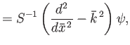
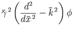
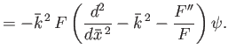
by the resistive-MHD equations, (7.182) and (7.183). We can simplify these equations,
making use of the fact that
, where the behavior of the plasma is governed
by the resistive-MHD equations, (7.182) and (7.183). We can simplify these equations,
making use of the fact that
 and
and
 in a
thin layer, to obtain the following layer equations:
in a
thin layer, to obtain the following layer equations:
Note that we have redefined the variables
,
 , and
, and  , such
that
, such
that
 ,
,
 ,
and
,
and
 . Here,
 |
(7.189) |
is the so-called hydromagnetic timescale.
The tearing mode stability problem reduces to solving the resistive-MHD layer equations,
(7.187) and (7.188), in the immediate vicinity of the interface,
, solving
the ideal-MHD equations, (7.185) and (7.186), everywhere else in the plasma, matching
the two solutions at the edge of the layer, and applying physical
boundary conditions as
 . This method
of solution was first described in a classic paper by Furth, Killeen, and
Rosenbluth (Furth, Killeen, and Rosenbluth 1963).
. This method
of solution was first described in a classic paper by Furth, Killeen, and
Rosenbluth (Furth, Killeen, and Rosenbluth 1963).
Let us consider the solution of the ideal-MHD equation (7.186) throughout
the bulk of the plasma. We could imagine launching a solution
 at large positive
 , which satisfies physical boundary conditions as
 , and integrating this solution to the right-hand boundary of
the resistive-MHD layer at
, and integrating this solution to the right-hand boundary of
the resistive-MHD layer at
 . Likewise, we could also launch
a solution at large negative
, which satisfies physical boundary
conditions as
. Likewise, we could also launch
a solution at large negative
, which satisfies physical boundary
conditions as
 , and integrate this solution to
the left-hand boundary of the resistive-MHD layer at
, and integrate this solution to
the left-hand boundary of the resistive-MHD layer at
 .
Maxwell's equations demand that
.
Maxwell's equations demand that  must be continuous on either side
of the layer.
Hence, we can multiply our two solutions by appropriate factors, so as to ensure that
matches to the left and right of the layer. This leaves
the function
undetermined
to an overall arbitrary multiplicative constant, just as we would expect in a
linear problem. In general,
must be continuous on either side
of the layer.
Hence, we can multiply our two solutions by appropriate factors, so as to ensure that
matches to the left and right of the layer. This leaves
the function
undetermined
to an overall arbitrary multiplicative constant, just as we would expect in a
linear problem. In general,
 is not continuous to the left and
right of the layer. Thus, the ideal solution can be characterized by the
real number
is not continuous to the left and
right of the layer. Thus, the ideal solution can be characterized by the
real number
![$\displaystyle {\mit\Delta}' = \left[\frac{1}{\psi}\frac{d\psi}{d\bar{x}}\right]_{\bar{x}=0_-}^{\bar{x}=0_+}:$](img2691.png) |
(7.190) |
that is, by the jump in the logarithmic derivative of
to the left and
right of the layer.
This parameter is known as the tearing stability index, and is solely
a property
of the plasma equilibrium, the wavenumber,  ,
and the boundary conditions imposed at infinity.
,
and the boundary conditions imposed at infinity.
The layer equations, (7.187) and (7.188), possess a trivial solution (
 ,
,
 , where
  is independent of
), and
a nontrivial solution for which
is independent of
), and
a nontrivial solution for which
 and
and
 .
The asymptotic behavior of the nontrivial solution at the
edge of the layer is
.
The asymptotic behavior of the nontrivial solution at the
edge of the layer is
where the parameter
 is determined by solving the
layer equations, subject to the previous boundary
conditions. Finally, the growth-rate,
, of the tearing instability is determined
by the matching criterion
is determined by solving the
layer equations, subject to the previous boundary
conditions. Finally, the growth-rate,
, of the tearing instability is determined
by the matching criterion
 |
(7.193) |
The layer equations, (7.187) and (7.188), can be solved in a fairly straightforward manner
in Fourier transform space. Let
where
 .
Equations (7.187) and (7.188) can be Fourier transformed, and the results combined, to
give
.
Equations (7.187) and (7.188) can be Fourier transformed, and the results combined, to
give
 |
(7.196) |
where
 |
(7.197) |
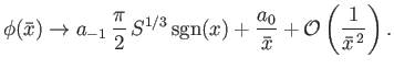
The most general small- asymptotic solution of Equation (7.196) is written
 |
(7.198) |
where  and
and  are independent of
, and it is assumed that
are independent of
, and it is assumed that  .
When inverse Fourier transformed, the previous expression leads to the
following expression for the asymptotic behavior of
at the edge of
the resistive-MHD layer (Erdéyli 1954):
.
When inverse Fourier transformed, the previous expression leads to the
following expression for the asymptotic behavior of
at the edge of
the resistive-MHD layer (Erdéyli 1954):
 |
(7.199) |
It follows from a comparison with Equations (7.191) and (7.192) that
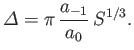 |
(7.200) |
Thus, the matching parameter
 is determined from the
small-
asymptotic behavior of the Fourier transformed layer solution.
is determined from the
small-
asymptotic behavior of the Fourier transformed layer solution.
Let us search for an unstable tearing mode, characterized by  . It is
convenient to assume that
. It is
convenient to assume that
 |
(7.201) |
This ordering, which is known as the constant-
approximation [because
it implies that
is approximately constant across the layer]
will be justified later on.
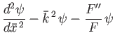
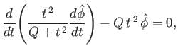
In the limit
 , Equation (7.196)
reduces to
, Equation (7.196)
reduces to
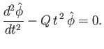 |
(7.202) |
The solution to this equation that is well behaved in the limit
 is written
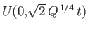 , where
 is a standard parabolic cylinder function (Abramowitz and Stegun 1965e). In the limit
 |
(7.203) |
we can make use of the standard small argument asymptotic expansion
of
to write the most general solution to Equation (7.196) in the
form (Abramowitz and Stegun 1965e)
![$\displaystyle \skew{3}\hat{\phi}(t) = A\left[ 1- 2 \,\frac{{\mit\Gamma}(3/4)}{{\mit\Gamma}(1/4)} \, Q^{\,1/4}\,t + {\cal O}(t^{\,2})\right].$](img2725.png) |
(7.204) |
Here,  is an arbitrary constant.
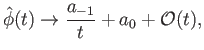
In the limit
 |
(7.205) |
Equation (7.196) reduces to
 |
(7.206) |
The most general solution to this equation is written
 |
(7.207) |
where  and
and  are arbitrary constants.
Matching coefficients between Equations (7.204) and (7.207) in the range of
satisfying the inequality (7.203) yields the following expression
for the most general solution to Equation (7.196) in the limit
are arbitrary constants.
Matching coefficients between Equations (7.204) and (7.207) in the range of
satisfying the inequality (7.203) yields the following expression
for the most general solution to Equation (7.196) in the limit
 :
:
![$\displaystyle \skew{3}\hat{\phi} = A\,\left[ 2\,\frac{{\mit\Gamma}(3/4)}{{\mit\Gamma}(1/4)} \, \frac{Q^{\,5/4}}{t} + 1 + {\cal O}(t)\right].$](img2730.png) |
(7.208) |
Finally, a comparison of Equations (7.198), (7.200), and (7.208)
gives the result
 |
(7.209) |
The asymptotic matching condition (7.193) can be combined with the previous
expression for
to give the tearing mode dispersion relation
![$\displaystyle \gamma = \left[\frac{{\mit\Gamma}(1/4)}{2\pi\,{\mit\Gamma}(3/4)}\right]^{\,4/5}\, \frac{({\mit\Delta}')^{\,4/5}}{\tau_H^{\,2/5}\,\tau_R^{\,3/5}}.$](img2732.png) |
(7.210) |
Here, use has been made of the definitions of
and  . According
to the dispersion relation, the tearing mode is unstable whenever
. According
to the dispersion relation, the tearing mode is unstable whenever
 , and grows on the hybrid timescale
 .
It is easily demonstrated that the tearing mode is stable whenever
.
It is easily demonstrated that the tearing mode is stable whenever
 .
According to Equations (7.193), (7.201), and (7.209), the constant-
approximation holds provided that
.
According to Equations (7.193), (7.201), and (7.209), the constant-
approximation holds provided that
 |
(7.211) |
that is, provided that the tearing mode does not become too
unstable.
According to Equation (7.202), the thickness of the resistive-MHD layer in
-space
is
 |
(7.212) |
It follows from Equations (7.194) and (7.195) that the thickness of the layer in
-space
is
 |
(7.213) |
When
 then
then
 , according to
Equation (7.210), giving
, according to
Equation (7.210), giving
 . It is clear, therefore, that if
the Lundquist number,
, is very large then the resistive-MHD layer centered
on the interface,
, is extremely narrow.
. It is clear, therefore, that if
the Lundquist number,
, is very large then the resistive-MHD layer centered
on the interface,
, is extremely narrow.
The timescale for magnetic flux to diffuse across a layer of thickness
 (in
-space) is [see Equation (7.180)]
(in
-space) is [see Equation (7.180)]
 |
(7.214) |
If
 |
(7.215) |
then the tearing mode grows on a timescale that is far longer than the
timescale on which magnetic flux diffuses across the resistive layer. In this case,
we would expect the normalized ``radial'' magnetic field,
, to be approximately
constant across the layer, because any non-uniformities in
would be
smoothed out via resistive diffusion. It follows from Equations (7.213) and (7.214)
that the constant-
approximation holds provided that
 |
(7.216) |
(i.e.,  ), which is in agreement with Equation (7.201).
Next: Nonlinear Tearing Mode Theory
Up: Magnetohydrodynamic Fluids
Previous: Magnetic Reconnection
Richard Fitzpatrick
2016-01-23