MHD Waves

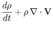
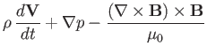
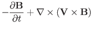
Let us investigate the small amplitude waves that propagate through a spatially uniform MHD plasma. We start by combining Equations (7.1)-(7.4) and (7.7)-(7.8) to form a closed set of equations:

$$\frac{d\rho}{dt} + \rho\,\nabla\cdot{\bf V} =0,$$ (7.22)

$$\rho\,\frac{d{\bf V}}{dt} + \nabla p - \frac{(\nabla\times{\bf B})\times {\bf B}}{\mu_0} ={\bf0},$$ (7.23)

$$-\frac{\partial{\bf B}}{\partial t}+ \nabla\times( {\bf V} \times {\bf B}) ={\bf0},$$ (7.24)

$$\frac{d}{dt}\!\left(\frac{p}{\rho^{\,{\mit\Gamma}}}\right) = 0.$$ (7.25)

Next, we linearize these equations (assuming, for the sake of simplicity, that the equilibrium flow velocity and equilibrium plasma current are both zero) to give

$$\frac{\partial\rho}{\partial t} + \rho_0\,\nabla\cdot{\bf V} =0,$$ (7.26)

$$\rho_0\,\frac{\partial {\bf V}}{\partial t} + \nabla p - \frac{(\nabla\times{\bf B})\times {\bf B}_0}{\mu_0} ={\bf0},$$ (7.27)

$$-\frac{\partial{\bf B}}{\partial t}+ \nabla\times( {\bf V} \times {\bf B}_0) ={\bf0},$$ (7.28)

$$\frac{\partial}{\partial t}\!\left(\frac{p}{p_0} - \frac{{\mit\Gamma}\,\rho}{\rho_0}\right) = 0.$$ (7.29)

Here, the subscript 0 denotes an equilibrium quantity. Perturbed quantities are written without subscripts. Of course, $\rho_0$ , $p_0$ , and ${\bf B}_0$ are constants in a spatially uniform plasma.

Let us search for wave-like solutions to Equations (7.26)-(7.29) in which perturbed quantities vary like $\exp[\,{\rm i}\,({\bf k}\cdot{\bf r}-\omega\,t)]$ . It follows that

$$-\omega\,\rho + \rho_0\,{\bf k}\cdot{\bf V} =0,$$ (7.30)

$$-\omega\,\rho_0\,{\bf V} + p\,{\bf k} - \frac{ ({\bf k}\times{\bf B})\times {\bf B}_0}{\mu_0} ={\bf0},$$ (7.31)

$$\omega\,{\bf B} + {\bf k}\times({\bf V}\times{\bf B}_0) ={\bf0},$$ (7.32)

$$-\omega\left(\frac{p}{p_0} - \frac{{\mit\Gamma}\,\rho}{\rho_0}\right) = 0.$$ (7.33)

Assuming that $\omega\neq 0$ , the previous equations yield

$$\rho = \rho_0\,\frac{{\bf k}\cdot{\bf V}}{\omega},$$ (7.34)

$$p ={\mit\Gamma}\,p_0\,\frac{{\bf k}\cdot{\bf V}}{\omega},$$ (7.35)

$${\bf B} = \frac{ ({\bf k}\cdot{\bf V})\,{\bf B}_0 - ({\bf k}\cdot{\bf B}_0)\,{\bf V}}{\omega}.$$ (7.36)

Substitution of these expressions into the linearized equation of motion, Equation (7.31), gives

$$\left[ \omega^2 - \frac{({\bf k}\cdot{\bf B}_0)^2}{\mu_0\,\rho_0} \right] {\bf V} = \left[ \left(\frac{{\mit\Gamma}\,p_0}{\rho_0} + \frac{B_0^{\,2}}{... ...{\bf k}\cdot{\bf B}_0)}{\mu_0\,\rho_0}\,{\bf B}_0 \right] ({\bf k}\cdot{\bf V})$$

$$- \frac{({\bf k}\cdot{\bf B}_0)\, ({\bf V}\cdot{\bf B}_0)}{\mu_0\,\rho_0} \,{\bf k}.$$ (7.37)

We can assume, without loss of generality, that the equilibrium magnetic field, ${\bf B}_0$ , is directed along the $z$ -axis, and that the wavevector, ${\bf k}$ , lies in the $x$ -$z$ plane. Let $\theta$ be the angle subtended between ${\bf B}_0$ and ${\bf k}$ . Equation (7.37) reduces to the eigenvalue equation

$$\left( \begin{array}{ccc} { \omega^2 - k^2\,V_A^{\,2} -k^2\,V_S^{... ...eft(\begin{array}{c}V_x\\ [0.5ex] V_y\\ [0.5ex] V_z\end{array}\right) = {\bf0}.$$ (7.38)

Here,

$$V_A = \sqrt{\frac{B_0^{\,2}}{\mu_0\,\rho_0}}$$ (7.39)

is the Alfvén speed, and

$$V_S = \sqrt{\frac{{\mit\Gamma}\,p_0}{\rho_0}}$$ (7.40)

is the sound speed. The solubility condition for Equation (7.38) is that the determinant of the square matrix is zero. This yields the dispersion relation

$$(\omega^2 - k^2\,V_A^{\,2}\,\cos^2\theta)\left[ \omega^4 - \omega... ...2\,(V_A^{\,2}+V_S^{\,2}) + k^4\,V_A^{\,2}\,V_S^{\,2}\,\cos^2\theta \right] = 0.$$ (7.41)

There are three independent roots of the previous dispersion relation, corresponding to the three different types of wave that can propagate through an MHD plasma. The first, and most obvious, root is

$$\omega = k\,V_A\,\cos\theta,$$ (7.42)

which has the associated eigenvector $(0,\,V_y,\, 0)$ . This root is characterized by both ${\bf k}\cdot{\bf V} =0$ and ${\bf V}\cdot {\bf B}_0=0$ . It immediately follows from Equations (7.34) and (7.35) that there is zero perturbation of the plasma density or pressure associated with the root. In fact, this particular root can easily be identified as the shear-Alfvén wave introduced in Section 5.8. The properties of the shear-Alfvén wave in a warm (i.e., non-zero pressure) plasma are unchanged from those found earlier in a cold plasma. Finally, because the shear-Alfvén wave only involves plasma motion perpendicular to the magnetic field, we would expect the dispersion relation (7.42) to hold good in a collisionless, as well as a collisional, plasma.

The remaining two roots of the dispersion relation (7.41) are written

$$\omega = k\,V_+,$$ (7.43)

and

$$\omega = k\,V_-,$$ (7.44)

respectively. Here,

$$V_\pm = \left\{\frac{1}{2}\left[V_A^{\,2} + V_S^{\,2} \pm \sqrt{ ... ...{\,2})^{\,2} - 4\, V_A^{\,2}\,V_S^{\,2}\,\cos^2\theta} \,\right]\right\}^{1/2}.$$ (7.45)

Note that $V_+\geq V_-$ . The first root is generally termed the fast magnetosonic wave, or fast wave, for short, whereas the second root is usually called the slow magnetosonic wave, or slow wave. The eigenvectors for these waves are $(V_x,\,0,\,V_z)$ . It follows that ${\bf k}\cdot{\bf V} \neq 0$ and ${\bf V}\cdot {\bf B}_0\neq0$ . Hence, these waves are associated with non-zero perturbations in the plasma density and pressure, and also involve plasma motion parallel, as well as perpendicular, to the magnetic field. The latter observation suggests that the dispersion relations (7.43) and (7.44) are likely to undergo significant modification in collisionless plasmas.

In order to better understand the nature of the fast and slow waves, let us consider the cold plasma limit, which is obtained by letting the sound speed, $V_S$ , tend to zero. In this limit, the slow wave ceases to exist (in fact, its phase-velocity tends to zero), whereas the dispersion relation for the fast wave reduces to

$$\omega = k\,V_A.$$ (7.46)

This can be identified as the dispersion relation for the compressional-Alfvén wave introduced in Section 5.8. Thus, we can identify the fast wave as the compressional-Alfvén wave modified by a non-zero plasma pressure.

In the limit $V_A\gg V_S$ , which is appropriate to low-$\beta$ plasmas (see Section 4.15), the dispersion relation for the slow wave reduces to

$$\omega \simeq k\,V_S\,\cos\theta.$$ (7.47)

This is actually the dispersion relation of a sound wave propagating along magnetic field-lines. Thus, in low-$\beta$ plasmas, the slow wave is a sound wave modified by the presence of the magnetic field.

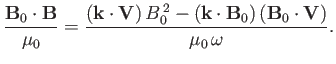
The distinction between the fast and slow waves can be further understood by comparing the signs of the wave-induced fluctuations in the plasma and magnetic pressures: $p$ and ${\bf B}_0\cdot {\bf B}/\mu_0$ , respectively. It follows from Equation (7.36) that

$$\frac{{\bf B}_0\cdot{\bf B}}{\mu_0} = \frac{({\bf k}\cdot{\bf V})\,B_0^{\,2} - ({\bf k}\cdot{\bf B}_0)\,({\bf B}_0\cdot{\bf V})} {\mu_0\,\omega}.$$ (7.48)

Now, the $z$ -component of Equation (7.31) yields

$$\omega\,\rho_0\,V_z = k\,\cos\theta\,p.$$ (7.49)

Combining Equations (7.35), (7.39), (7.40), (7.48), and (7.49), we obtain

$$\frac{{\bf B}_0\cdot{\bf B}}{\mu_0} =\frac{V_A^{\,2}}{V_S^{\,2}} \left(1-\frac{k^2\,V_S^{\,2}\,\cos^2\theta} {\omega^2}\right)p.$$ (7.50)

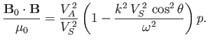
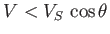
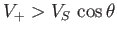
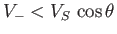Hence, $p$ and ${\bf B}_0\cdot {\bf B}/\mu_0$ have the same sign if $V>V_S \,\cos\theta$ , and the opposite sign if $V<V_S\,\cos\theta$ . Here, $V=\omega/k$ is the phase-velocity. It is straightforward to show that $V_+> V_S\,\cos\theta$ , and $V_-<V_S\,\cos\theta$ . Thus, we conclude that the plasma pressure and magnetic pressure fluctuations reinforce one another in the fast magnetosonic wave, whereas the fluctuations oppose one another in the slow magnetosonic wave.

Figure: Schematic diagram showing the variation of the phase velocities of the three MHD waves with direction of propagation in the $x$ -$z$ plane.

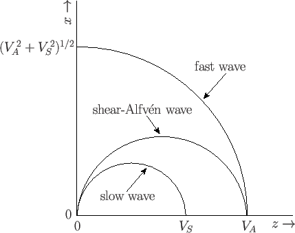Figure 7.1 shows the variation of the phase velocities of the three MHD waves with direction of propagation in the $x$ -$z$ plane for a low-$\beta$ plasma in which $V_S<V_A$ . It can be seen that the slow wave always has a smaller phase-velocity than the shear-Alfvén wave, which, in turn, always has a smaller phase-velocity than the fast wave.

The existence of MHD waves was first predicted theoretically by Alfvén (Alfvén 1942). These waves were subsequently observed in the laboratory--first in magnetized conducting fluids (e.g., mercury) (Lundquist 1949), and then in magnetized plasmas (Wilcox, Boley, and DeSilva 1960).