Gauge transformations

Electric and magnetic fields can be written in terms of scalar and vector potentials, as follows:

$${\bf E} = - \nabla\phi - \frac{\partial {\bf A}}{\partial t},$$ (385)

$${\bf B} = \nabla\times{\bf A}.$$ (386)

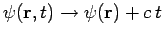
However, this prescription is not unique. There are many different potentials which can generate the same fields. We have come across this problem before. It is called gauge invariance. The most general transformation which leaves the ${\bf E}$ and ${\bf B}$ fields unchanged in Eqs. (385) and (386) is

$$\phi \rightarrow \phi +\frac{\partial \psi}{\partial t},$$ (387)

$${\bf A} \rightarrow {\bf A} - \nabla\psi.$$ (388)

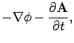
This is clearly a generalization of the gauge transformation which we found earlier for static fields:

$$\phi \rightarrow \phi +c,$$ (389)

$${\bf A} \rightarrow {\bf A} - \nabla\psi,$$ (390)

where $c$ is a constant. In fact, if $\psi({\bf r}, t)\rightarrow \psi({\bf r}) + c t$ then Eqs. (387) and (388) reduce to Eqs. (389) and (390).

We are free to choose the gauge so as to make our equations as simple as possible. As before, the most sensible gauge for the scalar potential is to make it go to zero at infinity:

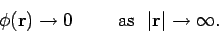$$\phi({\bf r}) \rightarrow 0\mbox{\hspace{1cm}as  $\vert{\bf r}\vert\rightarrow \infty$}.$$ (391)

For steady fields, we found that the optimum gauge for the vector potential was the so-called Coulomb gauge:

$$\nabla\cdot{\bf A} = 0.$$ (392)

We can still use this gauge for non-steady fields. The argument which we gave earlier (see Sect. 3.12), that it is always possible to transform away the divergence of a vector potential, remains valid. One of the nice features of the Coulomb gauge is that when we write the electric field,

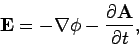$${\bf E} = -\nabla\phi - \frac{\partial {\bf A}}{\partial t},$$ (393)

we find that the part which is generated by charges (i.e., the first term on the right-hand side) is conservative, and the part induced by magnetic fields (i.e., the second term on the right-hand side) is purely solenoidal. Earlier on, we proved mathematically that a general vector field can be written as the sum of a conservative field and a solenoidal field (see Sect. 3.11). Now we are finding that when we split up the electric field in this manner the two fields have different physical origins: the conservative part of the field emanates from electric charges, whereas the solenoidal part is induced by magnetic fields.

Equation (393) can be combined with the field equation

$$\nabla\cdot {\bf E} = \frac{\rho}{\epsilon_0}$$ (394)

(which remains valid for non-steady fields) to give

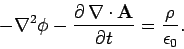$$-\nabla^2 \phi - \frac{\partial \nabla\cdot{\bf A}}{\partial t} = \frac{\rho}{\epsilon_0}.$$ (395)

With the Coulomb gauge condition, $\nabla\cdot {\bf A} = 0$, the above expression reduces to

$$\nabla^2\phi = -\frac{\rho}{\epsilon_0},$$ (396)

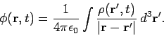
which is just Poisson's equation. Thus, we can immediately write down an expression for the scalar potential generated by non-steady fields. It is exactly the same as our previous expression for the scalar potential generated by steady fields, namely

$$\phi({\bf r},t)= \frac{1}{4\pi\epsilon_0} \int \frac{\rho({\bf r}',t)}{\vert{\bf r} - {\bf r}'\vert} d^3{\bf r}'.$$ (397)

However, this apparently simple result is extremely deceptive. Equation (397) is a typical action at a distance law. If the charge density changes suddenly at ${\bf r}'$ then the potential at ${\bf r}$ responds immediately. However, we shall see later that the full time-dependent Maxwell's equations only allow information to propagate at the speed of light (i.e., they do not violate relativity). How can these two statements be reconciled? The crucial point is that the scalar potential cannot be measured directly, it can only be inferred from the electric field. In the time-dependent case, there are two parts to the electric field: that part which comes from the scalar potential, and that part which comes from the vector potential [see Eq. (393)]. So, if the scalar potential responds immediately to some distance rearrangement of charge density it does not necessarily follow that the electric field also has an immediate response. What actually happens is that the change in the part of the electric field which comes from the scalar potential is balanced by an equal and opposite change in the part which comes from the vector potential, so that the overall electric field remains unchanged. This state of affairs persists at least until sufficient time has elapsed for a light signal to travel from the distant charges to the region in question. Thus, relativity is not violated, since it is the electric field, and not the scalar potential, which carries physically accessible information.

It is clear that the apparent action at a distance nature of Eq. (397) is highly misleading. This suggests, very strongly, that the Coulomb gauge is not the optimum gauge in the time-dependent case. A more sensible choice is the so called Lorentz gauge:

$$\nabla\cdot {\bf A} = -\epsilon_0 \mu_0 \frac{\partial \phi}{\partial t}.$$ (398)

It can be shown, by analogy with earlier arguments (see Sect. 3.12), that it is always possible to make a gauge transformation, at a given instance in time, such that the above equation is satisfied. Substituting the Lorentz gauge condition into Eq. (395), we obtain

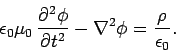$$\epsilon_0\mu_0 \frac{\partial^2\phi}{\partial t^2} - \nabla^2\phi = \frac{\rho} {\epsilon_0}.$$ (399)

It turns out that this is a three-dimensional wave equation in which information propagates at the speed of light. But, more of this later. Note that the magnetically induced part of the electric field (i.e., $-\partial {\bf A}/\partial t$) is not purely solenoidal in the Lorentz gauge. This is a slight disadvantage of the Lorentz gauge with respect to the Coulomb gauge. However, this disadvantage is more than offset by other advantages which will become apparent presently. Incidentally, the fact that the part of the electric field which we ascribe to magnetic induction changes when we change the gauge suggests that the separation of the field into magnetically induced and charge induced components is not unique in the general time-varying case (i.e., it is a convention).