The magnetic vector potential

Electric fields generated by stationary charges obey

$$\nabla\times{\bf E} = {\bf0}.$$ (315)

This immediately allows us to write

$${\bf E} = -\nabla \phi,$$ (316)

since the curl of a gradient is automatically zero. In fact, whenever we come across an irrotational vector field in physics we can always write it as the gradient of some scalar field. This is clearly a useful thing to do, since it enables us to replace a vector field by a much simpler scalar field. The quantity $\phi$ in the above equation is known as the electric scalar potential.

Magnetic fields generated by steady currents (and unsteady currents, for that matter) satisfy

$$\nabla \cdot {\bf B} = 0.$$ (317)

This immediately allows us to write

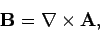$${\bf B} = \nabla\times{\bf A},$$ (318)

since the divergence of a curl is automatically zero. In fact, whenever we come across a solenoidal vector field in physics we can always write it as the curl of some other vector field. This is not an obviously useful thing to do, however, since it only allows us to replace one vector field by another. Nevertheless, Eq. (318) is one of the most useful equations we shall come across in this lecture course. The quantity ${\bf A}$ is known as the magnetic vector potential.

We know from Helmholtz's theorem that a vector field is fully specified by its divergence and its curl. The curl of the vector potential gives us the magnetic field via Eq. (318). However, the divergence of ${\bf A}$ has no physical significance. In fact, we are completely free to choose $\nabla\cdot{\bf A}$ to be whatever we like. Note that, according to Eq. (318), the magnetic field is invariant under the transformation

$${\bf A} \rightarrow {\bf A} - \nabla\psi.$$ (319)

In other words, the vector potential is undetermined to the gradient of a scalar field. This is just another way of saying that we are free to choose $\nabla\cdot{\bf A}$. Recall that the electric scalar potential is undetermined to an arbitrary additive constant, since the transformation

$$\phi \rightarrow \phi + c$$ (320)

leaves the electric field invariant in Eq. (316). The transformations (319) and (320) are examples of what mathematicians call gauge transformations. The choice of a particular function $\psi$ or a particular constant $c$ is referred to as a choice of the gauge. We are free to fix the gauge to be whatever we like. The most sensible choice is the one which makes our equations as simple as possible. The usual gauge for the scalar potential $\phi$ is such that $\phi\rightarrow 0$ at infinity. The usual gauge for ${\bf A}$ is such that

$$\nabla\cdot{\bf A} = 0.$$ (321)

This particular choice is known as the Coulomb gauge.

It is obvious that we can always add a constant to $\phi$ so as to make it zero at infinity. But it is not at all obvious that we can always perform a gauge transformation such as to make $\nabla\cdot{\bf A}$ zero. Suppose that we have found some vector field ${\bf A}$ whose curl gives the magnetic field but whose divergence in non-zero. Let

$$\nabla \cdot{\bf A} = v({\bf r}).$$ (322)

The question is, can we find a scalar field $\psi$ such that after we perform the gauge transformation (319) we are left with $\nabla\cdot {\bf A} = 0$. Taking the divergence of Eq. (319) it is clear that we need to find a function $\psi$ which satisfies

$$\nabla^2\psi = v.$$ (323)

But this is just Poisson's equation. We know that we can always find a unique solution of this equation (see Sect. 3.11). This proves that, in practice, we can always set the divergence of ${\bf A}$ equal to zero.

Let us again consider an infinite straight wire directed along the $z$-axis and carrying a current $I$. The magnetic field generated by such a wire is written

$${\bf B} = \frac{\mu_0 I}{2\pi} \left(\frac{-y}{r^2}, \frac{x}{r^2}, 0\right).$$ (324)

We wish to find a vector potential ${\bf A}$ whose curl is equal to the above magnetic field, and whose divergence is zero. It is not difficult to see that

$${\bf A} = -\frac{\mu_0 I}{4\pi} \left( 0, 0, \ln[x^2+y^2] \right)$$ (325)

fits the bill. Note that the vector potential is parallel to the direction of the current. This would seem to suggest that there is a more direct relationship between the vector potential and the current than there is between the magnetic field and the current. The potential is not very well-behaved on the $z$-axis, but this is just because we are dealing with an infinitely thin current.

Let us take the curl of Eq. (318). We find that

$$\nabla\times{\bf B} = \nabla\times\nabla\times {\bf A} = \nabla(\nabla\cdot{\bf A}) -\nabla^2{\bf A} = - \nabla^2{\bf A},$$ (326)

where use has been made of the Coulomb gauge condition (321). We can combine the above relation with the field equation (274) to give

$$\nabla^2{\bf A} = - \mu_0 {\bf j}.$$ (327)

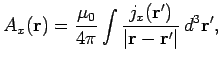
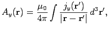
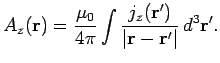
Writing this in component form, we obtain

$$\nabla^2 A_x = - \mu_0 j_x,$$ (328)

$$\nabla^2 A_y = - \mu_0 j_y,$$ (329)

$$\nabla^2 A_z = - \mu_0 j_z.$$ (330)

But, this is just Poisson's equation three times over. We can immediately write the unique solutions to the above equations:

$$A_x({\bf r}) = \frac{\mu_0}{4\pi} \int \frac{j_x({\bf r}')}{\vert{\bf r} - {\bf r}'\vert} d^3{\bf r}',$$ (331)

$$A_y({\bf r}) = \frac{\mu_0}{4\pi} \int \frac{j_y({\bf r}')}{\vert{\bf r} - {\bf r}'\vert} d^3{\bf r}',$$ (332)

$$A_z({\bf r}) = \frac{\mu_0}{4\pi} \int \frac{j_z({\bf r}')}{\vert{\bf r} - {\bf r}'\vert} d^3{\bf r}'.$$ (333)

These solutions can be recombined to form a single vector solution

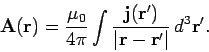$${\bf A}({\bf r}) = \frac{\mu_0}{4\pi} \int \frac{{\bf j}({\bf r}')}{\vert{\bf r} - {\bf r}'\vert} d^3{\bf r}'.$$ (334)

Of course, we have seen a equation like this before:

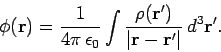$$\phi({\bf r}) = \frac{1}{4\pi \epsilon_0} \int \frac{ \rho({\bf r}')}{\vert{\bf r} - {\bf r}'\vert} d^3{\bf r}'.$$ (335)

Equations (334) and (335) are the unique solutions (given the arbitrary choice of gauge) to the field equations (279)-(282): they specify the magnetic vector and electric scalar potentials generated by a set of stationary charges, of charge density $\rho({\bf r})$, and a set of steady currents, of current density ${\bf j}({\bf r})$. Incidentally, we can prove that Eq. (334) satisfies the gauge condition $\nabla\cdot {\bf A} = 0$ by repeating the analysis of Eqs. (300)-(307) (with ${\bf W}\rightarrow{\bf A}$ and ${\bf C} \rightarrow \mu_0 {\bf j}$), and using the fact that $\nabla\cdot{\bf j} = 0$ for steady currents.