Next: The magnetic vector potential
Up: Time-independent Maxwell equations
Previous: Ampère's circuital law
Helmholtz's theorem
Let us now embark on a slight mathematical digression. Up to now, we have
only studied the
electric and magnetic fields generated by stationary charges and steady currents.
We have found that these fields are describable in terms of four field equations:
for electric fields,
and
for magnetic fields. There are no other field equations.
This strongly suggests that if we know the divergence and the curl of a vector field
then we know everything there is to know about the field. In fact, this is the
case. There is a mathematical theorem which sums this up. It is called
Helmholtz's theorem after the German polymath Hermann Ludwig Ferdinand von
Helmholtz.
Let us start with scalar fields. Field equations are a type of differential equation:
i.e., they deal with the infinitesimal differences in quantities between neighbouring
points. The question is, what
differential equation completely specifies a
scalar field? This is easy. Suppose that we have a scalar field  and a field equation which tells us the gradient of this field at all points:
something like
and a field equation which tells us the gradient of this field at all points:
something like
 |
(283) |
where
 is a vector field. Note that
we need
is a vector field. Note that
we need
 for self consistency, since the curl of a gradient is automatically zero.
The above equation completely
specifies once we are given the value of the field at a single
point,
for self consistency, since the curl of a gradient is automatically zero.
The above equation completely
specifies once we are given the value of the field at a single
point,  (say). Thus,
 |
(284) |
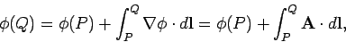
where  is a general point. The fact that
means
that
is a general point. The fact that
means
that  is a conservative field, which guarantees that the above
equation gives a unique value for at a general point in space.
is a conservative field, which guarantees that the above
equation gives a unique value for at a general point in space.
Suppose that we have a vector field  . How many differential equations
do we need to completely specify this field? Hopefully, we only need two: one
giving the divergence of the field, and one giving its curl. Let us
test this hypothesis. Suppose that we have two field equations:
. How many differential equations
do we need to completely specify this field? Hopefully, we only need two: one
giving the divergence of the field, and one giving its curl. Let us
test this hypothesis. Suppose that we have two field equations:
 |
|
|
(285) |
 |
|
|
(286) |
where  is a scalar field and
  is a vector field.
For self-consistency, we need
is a vector field.
For self-consistency, we need
 |
(287) |
since the divergence of a curl is automatically zero. The question is, do these
two field equations plus some suitable boundary conditions completely specify
? Suppose that we write
 |
(288) |
In other words, we are saying that a general field is the sum of
a conservative field,  , and a solenoidal field,
 .
This sounds plausible, but it remains to be proved.
Let us start by taking the divergence of the above equation, and making use of
Eq. (285). We get
.
This sounds plausible, but it remains to be proved.
Let us start by taking the divergence of the above equation, and making use of
Eq. (285). We get
 |
(289) |
Note that the vector field  does not figure in this equation, because
the divergence of a curl is automatically zero. Let us now take the curl of
Eq. (288):
does not figure in this equation, because
the divergence of a curl is automatically zero. Let us now take the curl of
Eq. (288):
 |
(290) |
Here, we assume that the divergence of is zero. This is another thing
which remains to be proved. Note that the scalar field  does not figure in
this equation, because the curl of a divergence is automatically zero.
Using Eq. (286), we
get
does not figure in
this equation, because the curl of a divergence is automatically zero.
Using Eq. (286), we
get
So, we have transformed our problem into four differential equations, Eq. (289)
and Eqs. (291)-(293), which
we need to solve. Let us look at these equations. We immediately notice that
they all have exactly the same form. In fact, they are all versions of Poisson's
equation. We can now make use of a principle made famous by Richard P. Feynman:
``the same equations have the same solutions.'' Recall that earlier on we
came across the following equation:
 |
(294) |
where is the electrostatic potential and  is the charge density.
We proved that the solution to this equation, with the boundary condition that
goes to zero at infinity, is
is the charge density.
We proved that the solution to this equation, with the boundary condition that
goes to zero at infinity, is
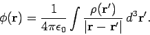 |
(295) |
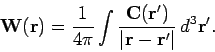
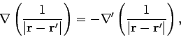
Well, if the same equations have the same solutions, and Eq. (295) is the solution
to Eq. (294), then we can immediately write down the solutions to
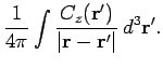
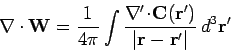
Eq. (289) and Eqs. (291)-(293). We get
 |
(296) |
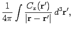
and
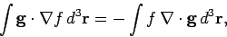
The last three equations can be combined to form a single vector equation:
 |
(300) |
We assumed earlier that
 . Let us check to
see if this is true. Note that
. Let us check to
see if this is true. Note that
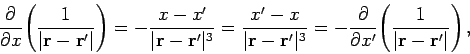 |
(301) |
which implies that
 |
(302) |
where  is the operator
 . Taking the divergence of Eq. (300), and making use of
the above relation, we obtain
. Taking the divergence of Eq. (300), and making use of
the above relation, we obtain
 |
(303) |
Now
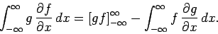 |
(304) |
However, if
 as
as
 then we can neglect the
first term on the right-hand side of the above equation and write
then we can neglect the
first term on the right-hand side of the above equation and write
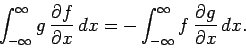 |
(305) |
A simple generalization of this result yields
 |
(306) |
provided that
 as
as
 , etc.
Thus, we can
deduce that
, etc.
Thus, we can
deduce that
 |
(307) |
from Eq. (303), provided
 is bounded as
. However, we have already shown that
is bounded as
. However, we have already shown that
 from self-consistency arguments, so the above equation
implies that
, which is the desired result.
from self-consistency arguments, so the above equation
implies that
, which is the desired result.
We have constructed a vector field which satisfies Eqs. (285) and (286)
and behaves sensibly at infinity: i.e.,
 as
. But, is our solution the only possible solution
of Eqs. (285) and (286) with sensible boundary conditions at infinity? Another way of posing
this question is to ask whether there are any solutions of
as
. But, is our solution the only possible solution
of Eqs. (285) and (286) with sensible boundary conditions at infinity? Another way of posing
this question is to ask whether there are any solutions of
 |
(308) |
where  denotes
  ,
,  , or
, or  , which are bounded at infinity. If there are
then we are in trouble, because we can take our solution and add to it an
arbitrary amount of a vector field with zero divergence and zero curl, and thereby
obtain another solution which also satisfies physical boundary conditions.
This would imply that our solution is not unique. In other words, it is not
possible to unambiguously reconstruct a vector field given its divergence,
its curl, and physical boundary conditions. Fortunately, the equation
, which are bounded at infinity. If there are
then we are in trouble, because we can take our solution and add to it an
arbitrary amount of a vector field with zero divergence and zero curl, and thereby
obtain another solution which also satisfies physical boundary conditions.
This would imply that our solution is not unique. In other words, it is not
possible to unambiguously reconstruct a vector field given its divergence,
its curl, and physical boundary conditions. Fortunately, the equation
 |
(309) |
which is called Laplace's equation, has a very nice property: its solutions are
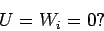
unique. That is, if we can find a solution to Laplace's equation
which satisfies the boundary conditions then we are guaranteed that this is
the only solution. We shall prove this later on in the course.
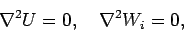
Well, let us invent some solutions to Eqs. (308) which are bounded at infinity.
How about
 |
(310) |
These solutions certainly satisfy Laplace's equation, and are well-behaved
at infinity. Because the solutions to Laplace's equations are unique, we know
that Eqs. (310) are the only solutions to Eqs. (308).
This means that there is no vector field which satisfies physical boundary
equations at infinity and has zero divergence and zero curl. In other words, our
solution to Eqs. (285) and (286) is the only solution. Thus, we have
unambiguously reconstructed the vector field given its divergence, its
curl, and sensible boundary conditions at infinity. This is Helmholtz's theorem.
We have just proved a number of very useful, and also very important, points.
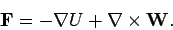
First, according to Eq. (288), a general vector field can be written as the
sum of a conservative field and a solenoidal field. Thus, we ought to be able
to write electric and magnetic fields in this form. Second, a general vector
field which is zero at infinity is completely specified once its divergence
and its curl are given. Thus, we can guess that the laws of electromagnetism
can be written as four field equations,
without knowing the first thing about electromagnetism (other than the fact that
it deals with two vector fields). Of course,
Eqs. (279)-(282) are of
exactly this form. We also know that there are only four field equations, since
the above equations are sufficient to completely reconstruct both  and
and
 . Furthermore, we know that we can solve the field equations without
even knowing what the right-hand sides look like. After all, we solved Eqs. (285)-(286)
for completely general right-hand sides. [Actually, the right-hand sides have
to go to zero at infinity, otherwise integrals like Eq. (296) blow up.]
We also know that any solutions we find are unique. In other words, there is only
one possible steady
electric and magnetic field which can be generated by a given set of
stationary charges and steady currents. The third thing which we proved was that
if the right-hand sides of the above field equations are all zero then
the only physical solution is
. Furthermore, we know that we can solve the field equations without
even knowing what the right-hand sides look like. After all, we solved Eqs. (285)-(286)
for completely general right-hand sides. [Actually, the right-hand sides have
to go to zero at infinity, otherwise integrals like Eq. (296) blow up.]
We also know that any solutions we find are unique. In other words, there is only
one possible steady
electric and magnetic field which can be generated by a given set of
stationary charges and steady currents. The third thing which we proved was that
if the right-hand sides of the above field equations are all zero then
the only physical solution is
 . This implies
that steady electric and magnetic fields cannot generate themselves.
Instead, they have to be generated by stationary charges and
steady currents. So, if we come across a steady electric field we know that if
we trace the field-lines back we shall eventually find a charge.
Likewise, a steady magnetic field implies that there is a steady
current flowing somewhere. All of these results follow from vector field theory
(i.e., from the general properties of fields in three-dimensional space), prior to
any investigation of electromagnetism.
. This implies
that steady electric and magnetic fields cannot generate themselves.
Instead, they have to be generated by stationary charges and
steady currents. So, if we come across a steady electric field we know that if
we trace the field-lines back we shall eventually find a charge.
Likewise, a steady magnetic field implies that there is a steady
current flowing somewhere. All of these results follow from vector field theory
(i.e., from the general properties of fields in three-dimensional space), prior to
any investigation of electromagnetism.
Next: The magnetic vector potential
Up: Time-independent Maxwell equations
Previous: Ampère's circuital law
Richard Fitzpatrick
2006-02-02