Effect of terrestrial oblateness on artificial satellite orbits
Consider a non-rotating (with respect to the distant stars) frame of reference whose origin coincides with the center of the Earth.
Such a frame can be regarded as approximately inertial when we consider orbital motion in the Earth's immediate vicinity.
Let  ,
,  ,
,  be a Cartesian coordinate system in the said reference frame that is orientated such that its
-axis is aligned with the Earth's (approximately) constant axis of rotation (with the terrestrial north pole lying at positive ).
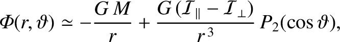
As we saw in Section 8.9, the gravitational potential in the immediate vicinity of the
Earth can be written
be a Cartesian coordinate system in the said reference frame that is orientated such that its
-axis is aligned with the Earth's (approximately) constant axis of rotation (with the terrestrial north pole lying at positive ).
As we saw in Section 8.9, the gravitational potential in the immediate vicinity of the
Earth can be written
 |
(10.110) |
where  is the Earth's mass,
 its moment of inertia about the -axis, and
 its moment of inertia about an axis lying in the - plane. Here,
 and
and
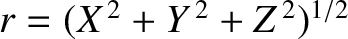
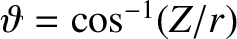 are standard spherical coordinates. The first term on the right-hand side of the
preceding expression is the monopole gravitational potential that would result were the Earth spherically symmetric.
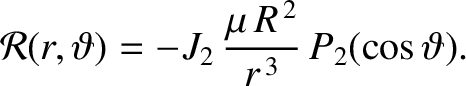
The second term is the small quadrupole correction to this potential generated by the Earth's slight oblateness. (See Section 6.5.)
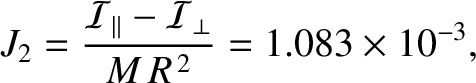
It is conventional to parameterize this correction in terms of the dimensionless quantity (Yoder 1995)
are standard spherical coordinates. The first term on the right-hand side of the
preceding expression is the monopole gravitational potential that would result were the Earth spherically symmetric.
The second term is the small quadrupole correction to this potential generated by the Earth's slight oblateness. (See Section 6.5.)
It is conventional to parameterize this correction in terms of the dimensionless quantity (Yoder 1995)
 |
(10.111) |
where  is the Earth's equatorial radius.
Hence, Equation (10.110) can be written
is the Earth's equatorial radius.
Hence, Equation (10.110) can be written
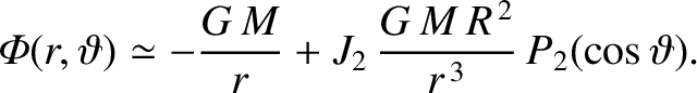 |
(10.112) |
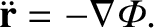
Consider an artificial satellite in orbit around the Earth. The satellite's equation of motion in our approximately
inertial geocentric reference frame takes the form
 |
(10.113) |
This can be combined with Equation (10.112) to give
 |
(10.114) |
where  , and
, and
 |
(10.115) |
Note that the preceding expression has exactly the same form as the canonical equation of motion, Equation (G.2),
that is the starting point for orbital perturbation theory. In particular,
 is the disturbing function that describes the perturbation to the Keplerian orbit of the satellite
due to the Earth's small quadrupole gravitational field.
is the disturbing function that describes the perturbation to the Keplerian orbit of the satellite
due to the Earth's small quadrupole gravitational field.
Let the satellite's osculating orbital elements be the major radius,  ; the time of perigee passage,
  ; the
eccentricity,
; the
eccentricity,  ; the inclination (to the Earth's equatorial plane),
  ; the argument of the perigee,
  ;
and the longitude of the ascending node (measured with respect to the vernal equinox),
;
and the longitude of the ascending node (measured with respect to the vernal equinox),
 . (See Section 4.12.) Actually, it is
more convenient to replace by the mean anomaly,
. (See Section 4.12.) Actually, it is
more convenient to replace by the mean anomaly,
 , where
 is the
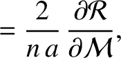
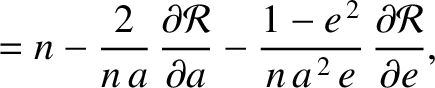
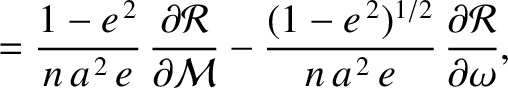
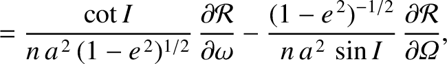
(unperturbed) mean orbital angular velocity. According to standard orbital perturbation theory, the time evolution of the satellite's
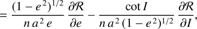
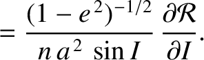
orbital elements is governed by the Lagrange planetary equations which, for the particular set of elements under consideration,
take the form (see Section G.6)
is the
(unperturbed) mean orbital angular velocity. According to standard orbital perturbation theory, the time evolution of the satellite's
orbital elements is governed by the Lagrange planetary equations which, for the particular set of elements under consideration,
take the form (see Section G.6)
According to Equation (4.74),
 |
(10.122) |
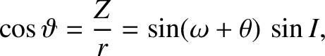
where  is the satellite's true anomaly. Thus, expression (10.115) can be written
![$\displaystyle {\cal R} = \frac{J_2}{2}\,\frac{\mu\,R^{\,2}}{r^{\,3}}\left[1-\frac{3}{2}\,\sin^2 I + \frac{3}{2}\,\sin^2 I\,\cos(2\,\omega+2\,\theta)\right].$](img2706.png) |
(10.123) |
We are primarily interested in the secular evolution of the satellite's orbital elements; that is, the evolution
on timescales much longer than the orbital period. We can concentrate on this evolution, and filter out any
relatively short-term oscillations in the elements, by averaging the disturbing function over an orbital period.
In other words, in Equations (10.116)–(10.121), we need to replace  by
by
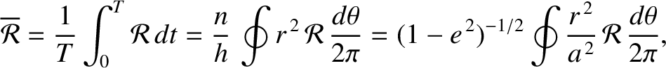 |
(10.124) |
where 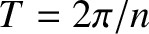 . Here, we have made use of the fact that
 is a
constant of the motion in a Keplerian
orbit. (See Chapter 4.) A Keplerian orbit is also characterized by
is a
constant of the motion in a Keplerian
orbit. (See Chapter 4.) A Keplerian orbit is also characterized by
 . Hence, the
previous two equations can be combined to give
. Hence, the
previous two equations can be combined to give
 |
![$\displaystyle = \frac{J_2}{2}\,\frac{\mu\,R^{\,2}}{a^{\,3}}\,(1-e^{\,2})^{-3/2}...
... + \frac{3}{2}\,\sin^2 I\,\cos(2\,\omega+2\,\theta)\right]\frac{d\theta}{2\pi},$](img2713.png) |
|
| |
|
(10.125) |
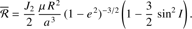 |
(10.126) |
Substitution of this expression into Equations (10.116), (10.118), and (10.119) (recalling that we are replacing
by
 ) reveals that there is no secular evolution of the satellite's orbital
major radius, , eccentricity, , and inclination, , due to the Earth's oblateness (because
does
not depend on
) reveals that there is no secular evolution of the satellite's orbital
major radius, , eccentricity, , and inclination, , due to the Earth's oblateness (because
does
not depend on  , , or
). On the other
hand, according to Equations (10.120) and (10.121), the oblateness causes the
satellite's perigee and ascending node to precess at the constant rates
, , or
). On the other
hand, according to Equations (10.120) and (10.121), the oblateness causes the
satellite's perigee and ascending node to precess at the constant rates
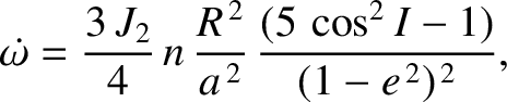 |
(10.127) |
and
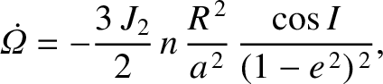 |
(10.128) |
respectively. These formulae suggest that the precession of the ascending node is always
in the opposite sense to the orbital motion; that is, it is retrograde. Note, however, that the
ascending node remains fixed in the special case of a so-called polar orbit
that passes over the terrestrial poles (i.e.,  ). The formulae also suggest that
the perigee precesses in a prograde fashion when
). The formulae also suggest that
the perigee precesses in a prograde fashion when
 , in a retrograde fashion when
 , and
remains fixed when
, and
remains fixed when
 . In other words, the perigee of an orbit lying in the Earth's equatorial plane
precesses in the same direction as the orbital motion, the perigee of a polar
orbit precesses in the opposite direction, and the perigee of an orbit that is inclined at the
critical angle of
. In other words, the perigee of an orbit lying in the Earth's equatorial plane
precesses in the same direction as the orbital motion, the perigee of a polar
orbit precesses in the opposite direction, and the perigee of an orbit that is inclined at the
critical angle of
 to the Earth's equatorial plane does not precess at all.
Finally, substitution of expression (10.126) into Equation (10.117) reveals that
to the Earth's equatorial plane does not precess at all.
Finally, substitution of expression (10.126) into Equation (10.117) reveals that
![$\displaystyle \frac{d{\cal M}}{dt} =n\left[1+\frac{3\,J_2}{2}\left(\frac{R}{a}\right)^2(1-e^{\,2})^{-3/2}\left(1-\frac{3}{2}\,\sin^2 I\right)\right].$](img2723.png) |
(10.129) |
We conclude that the Earth's oblateness causes the mean angular velocity of an orbiting satellite (which, by definition, is equal to
 )
to slightly exceed the Keplerian value
for low inclination orbits that satisfy
)
to slightly exceed the Keplerian value
for low inclination orbits that satisfy
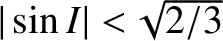 , to be slightly less than the
Keplerian value for high inclination orbits such that
, to be slightly less than the
Keplerian value for high inclination orbits such that
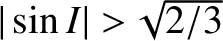 , and to exactly equal the Keplerian value when
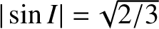 .
.
It should be noted that the dimensionless quadrupole moment of the Earth's gravitational field,  , (as well as higher-order
coefficients such as
, (as well as higher-order
coefficients such as  ; see Exercise 3) is most accurately determined via observations of the precession rates of the perigees and ascending
nodes of orbiting satellites.
; see Exercise 3) is most accurately determined via observations of the precession rates of the perigees and ascending
nodes of orbiting satellites.